Mean in Excel: 7 Core Functions & Pro Techniques

You're probably in a familiar spot. A manager asks for the average sales, average order value, or average score in a workbook that looks clean at first glance. Then you notice a giant outlier, a few blank cells, some text notes in the middle of the column, and maybe a stray TRUE/FALSE value from a prior import.

That's where mean in excel stops being a beginner topic and becomes an accuracy topic. The formula is easy. The judgment behind it is what makes your analysis reliable.

1 Reason Why the Simple Average Can Be Misleading

Users often start with =AVERAGE(range), and that's the right starting point. AVERAGE has been part of Excel since the first version in 1985, and more advanced options like AVERAGEIF and AVERAGEIFS arrived in Excel 2007. They matter because filtering average calculations is part of routine reporting for over 70% of Excel users, according to Ablebits' overview of mean, median, and mode in Excel.

The problem isn't the function itself. The problem is assuming that every dataset deserves the same kind of average.

Say you're asked for average monthly sales. If one month includes a one-off enterprise deal that dwarfs the rest, the average may rise sharply and suggest normal performance is stronger than it really is. If your range contains notes, blanks, or imported values that look numeric but aren't, your result may also reflect Excel's rules instead of your business reality.

Practical rule: The right average starts with a question, not a formula. Ask what you want the number to represent before you calculate it.

That's why strong analysts don't treat the mean as a button-click. They treat it as a choice about representation. Sometimes you want the arithmetic mean. Sometimes you want a filtered mean. Sometimes the better answer isn't mean at all.

If your next step is turning that result into a chart or dashboard, pair the calculation with clear presentation. A solid guide to Excel data visualization for business reporting helps you avoid building a polished chart around a weak average.

The 3 Core Measures of Central Tendency Explained

When people say “average,” they often mean one of three different things. Excel gives you tools for all three, but each one tells a different story.

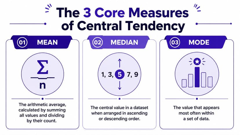
Mean tells you the arithmetic center

The mean adds all values and divides by the count. For the dataset {1, 2, 2, 3, 4, 6}, the mean is 3, as shown in Statistics By Jim's descriptive statistics guide for Excel.

In Excel, that's:

=AVERAGE(A1:A6)

Use mean when the values are reasonably balanced and you want every number to contribute equally.

Median shows the middle value

The median is the middle number after sorting the data. In the same dataset, the median is 2.5.

In Excel:

=MEDIAN(A1:A6)

Median becomes valuable when one or two values are extreme. Think of home prices in a neighborhood. If most homes cluster in one price band and one mansion sells for far more, the median often gives a more typical picture than the mean.

Mode identifies the most frequent value

The mode is the value that appears most often. In {1, 2, 2, 3, 4, 6}, the mode is 2.

In Excel:

=MODE.SNGL(A1:A6)

This is useful when repetition matters more than magnitude. Product sizes, repeated error codes, and most common customer choices are common examples.

A quick side by side comparison

Measure	Excel function	What it answers	Best use case
Mean	AVERAGE	What is the arithmetic average?	Balanced numeric data
Median	MEDIAN	What is the middle value?	Skewed data with outliers
Mode	MODE.SNGL	What value appears most often?	Frequency-based analysis

Income is a classic reason this distinction matters. In skewed data, the mean can exceed the median by 20-50%, which can distort what looks “typical,” as noted in this Excel-focused explanation of descriptive statistics and the source above.

If one value can dominate the story, check the median before you trust the mean.

5 Essential Functions to Calculate Mean in Excel

The biggest jump in skill comes when you stop using one average formula for every situation. Excel has several average functions because real worksheets aren't uniform.

1 AVERAGE for standard numeric data

Syntax:

=AVERAGE(number1, [number2], ...)

Most of the time, you'll use a range:

=AVERAGE(B2:B13)

This adds the numeric cells and divides by the number of numeric cells. It ignores blank cells and text entries in references.

If your column contains only valid numbers, this is the cleanest choice. It's also the easiest formula to audit because most Excel users understand it immediately.

2 AVERAGEA for mixed data

Syntax:

=AVERAGEA(value1, [value2], ...)

This distinction often trips up users. AVERAGEA does not behave like AVERAGE.

For the range {1,2,3,"text",TRUE}, =AVERAGE() returns 2.0, while =AVERAGEA() returns 1.4, because AVERAGEA counts TRUE as 1 and text as 0, according to Microsoft's AVERAGE function documentation.

That means AVERAGEA is useful when logical values are intentionally part of your scoring model, but risky when they appear accidentally.

How these functions treat different cell types

Function	Handles Numbers	Handles Blanks	Handles Text	Handles TRUE/FALSE
AVERAGE	Yes	Ignores blanks	Ignores text in references	Ignores logicals in references
AVERAGEA	Yes	Counts blanks differently in evaluation context	Treats text as 0	Treats TRUE as 1 and FALSE as 0
AVERAGEIF	Yes	Depends on criteria range and average range	Can use text in criteria	Logical handling depends on data structure
AVERAGEIFS	Yes	Depends on criteria ranges and average range	Can use text in criteria	Logical handling depends on data structure
TRIMMEAN	Yes	Works on numeric array input	Non-numeric entries should be cleaned first	Not intended for mixed logical analysis

3 AVERAGEIF for one condition

Syntax:

=AVERAGEIF(range, criteria, [average_range])

Use this when you want the mean for values matching one rule.

Example:

=AVERAGEIF(A2:A20,"North",B2:B20)

This calculates the average of values in B2:B20 only where A2:A20 equals "North".

That's useful for questions like:

• Regional reporting: average sales for one territory
• Status filtering: average delivery time for completed orders
• Simple thresholds: average score above a pass mark

If you're still building confidence with formula structure, a practical guide on how to make a formula in Excel helps with range logic and references.

4 AVERAGEIFS for multiple conditions

Syntax:

=AVERAGEIFS(average_range, criteria_range1, criteria1, [criteria_range2, criteria2], ...)

This is the workhorse for business reporting.

Example:

=AVERAGEIFS(C2:C100,A2:A100,"North",B2:B100,"Q1")

This returns the average from column C only for rows where region is North and quarter is Q1.

Use AVERAGEIFS when one condition isn't enough. Most analysts need averages by region, period, product line, owner, or status. This function keeps that logic inside one readable formula.

A quick video can help if you learn better by seeing formulas built in a sheet:

5 TRIMMEAN for outlier control

Syntax:

=TRIMMEAN(array, percent)

Example:

=TRIMMEAN(B2:B21,0.2)

This removes a percentage of data points from the top and bottom before calculating the mean. It's useful when a few extreme values make the regular average unrepresentative.

Suppose you're averaging transaction values and one refund reversal creates an unusually large negative value while one annual contract creates an unusually large positive value. TRIMMEAN gives you a center that better reflects the middle of your real activity.

Why this matters: If your average changes dramatically after trimming extremes, your dataset probably needs more interpretation before it goes into a report.

3 Advanced Techniques for More Precise Averages

Basic formulas answer basic questions. Better analysis often needs more context than a simple arithmetic mean can provide.

Weighted mean when values don't matter equally

A plain average assumes each value has the same importance. That's often false.

If product A has a rating of 5 from a handful of reviews and product B has a rating of 4 from many more reviews, you need a weighted mean. In Excel, the classic formula is:

=SUMPRODUCT(B2:B6,C2:C6)/SUM(C2:C6)

If B2:B6 contains ratings and C2:C6 contains review counts, SUMPRODUCT multiplies each rating by its weight, and SUM adds the weights. The result is an average that reflects volume.

This same logic works for average price by units sold, average margin by revenue contribution, or average score by response count. If you want a dedicated walkthrough, this guide to calculating weighted average in Excel is a good companion.

Moving average for trend analysis

A moving average smooths short-term volatility so you can see the underlying pattern.

A simple example for a three-period moving average might be:

=AVERAGE(B2:B4)

Then copy the formula downward so each row averages the current period and the prior ones. Sales teams use this to reduce monthly noise. Finance teams use it to track trend direction without overreacting to one unusual period.

If you work with time-series data or technical charts, Alpha Scala's technical indicator education gives useful context on how moving averages are interpreted in practice.

Geometric mean for growth rates

Arithmetic mean is not always the right mean. Growth rates are a prime example.

For compound annual growth work, using the arithmetic mean can overestimate results by 12-18% compared to GEOMEAN, according to GeeksforGeeks' Excel explanation of mean functions.

In Excel, use:

=GEOMEAN(B2:B6)

This matters when the numbers represent multiplicative change rather than simple additive values. Revenue growth factors, return multipliers, and indexed performance data usually fit this pattern.

PivotTables for category averages

Sometimes the best technique isn't a formula in a cell. It's a PivotTable.

Drop a category field into Rows, a metric into Values, then change the Value Field Settings from Sum to Average. Excel will calculate category-level means quickly and let you regroup, filter, and compare without rewriting formulas.

That's especially useful when you need average sales by region, average discount by rep, or average resolution time by support queue.

A PivotTable is often the fastest way to answer “average by category” because it separates calculation from layout.

Troubleshooting 4 Common Mean Calculation Errors

Averages go wrong for predictable reasons. Most aren't advanced Excel problems. They're data quality problems disguised as formula problems.

More than 40% of forum questions about Excel means involve errors from non-numeric data, blanks, or logical values, based on the referenced forum-pattern summary in this background tutorial source. That tracks with what analysts see every day in imported CSVs and copied reports.

1 Text formatted like numbers

A cell may show 250, but Excel may store it as text. If that happens, AVERAGE can ignore it.

Common clues include left-aligned numbers, green error triangles, or values imported from another system. Fix these before averaging. Use Text to Columns, multiply by 1 in a helper column, or wrap with VALUE() if needed.

2 Blanks versus zeros

Blank cells and zero cells are not the same thing.

If a zero means “no sales occurred,” it belongs in the average. If a blank means “data not collected yet,” it may not. Analysts often mix these meanings in the same report and end up with a misleading result.

Use a quick check:

• Blank cells: often indicate missing data
• Zero values: indicate an actual measured value of zero
• Best practice: confirm the business meaning before calculating

3 The #DIV/0! error

This happens when Excel tries to divide by zero because there are no valid numeric entries in the range being averaged.

For example, if a filtered range contains only text or only empty cells, AVERAGE has nothing to divide by. One practical workaround is to clean the data first. Another is to use error-aware logic around the formula.

For ranges that may contain errors, many analysts also use:

=AGGREGATE(1,6,B2:B20)

Here, 1 tells Excel to calculate an average, and 6 tells it to ignore errors. This is especially helpful in operational sheets where one bad formula result shouldn't break the whole summary.

4 Outliers that distort the story

A formula can be technically correct and still analytically weak.

One unusually large contract, one one-time write-off, or one imported anomaly can push the mean far from the center of the normal data. In that case, review the distribution, filter obvious anomalies if justified, or test TRIMMEAN.

Check whether the mean matches the story you know about the business. If it doesn't, inspect the rows before you present the number.

A simple troubleshooting flow works well:

1. Inspect data types and convert text numbers.
2. Separate blanks from zeros based on meaning.
3. Handle formula errors before averaging.
4. Test sensitivity to outliers using filtering or trimmed methods.

Automate All 15+ Mean Calculations with 1 Command

After you've worked through standard mean, conditional mean, trimmed mean, weighted mean, moving average, and category averages, a pattern appears. The hard part isn't one formula. It's the chain of steps around it.

In a real workbook, you don't just calculate a mean. You clean imported values, detect text stored as numbers, decide whether blanks should count, filter categories, build summaries, and often chart the result. That's where AI inside Excel becomes practical, not flashy.

Instead of writing every formula manually, you can use a natural-language workflow to do the full job in one pass. A command like “calculate the weighted average sales by category, exclude extreme values, and create a report” reflects how analysts think. The tool handles the mechanics.

This is why automation is becoming part of daily Excel work. It reduces repetitive setup, lowers formula mistakes, and makes complex average analysis easier to reproduce across files. If you're exploring that shift, this article on Excel automation workflows is a useful next read.

The key idea is simple. Manual formula skill still matters, because you need to judge whether the result makes sense. But once you understand the logic, you don't need to spend your time rebuilding the same mean calculations every week.

Your 2-Minute Recap on Mastering Excel Averages

Mean in excel looks simple until your worksheet gets messy. Then the difference between a solid analyst and a frustrated one usually comes down to one habit. Choosing the right calculation for the job.

Use AVERAGE for clean numeric data. Switch to AVERAGEIF or AVERAGEIFS when the average should reflect conditions. Reach for AVERAGEA only when you intentionally want text and logical values to affect the result. Use TRIMMEAN, weighted averages, moving averages, or GEOMEAN when the business question requires more precision.

You also need to check the data before trusting the answer. Text masquerading as numbers, blanks, zeros, formula errors, and outliers can all change the story.

That's a major upgrade in skill. You're no longer just calculating an average. You're deciding what “average” should mean for the problem in front of you.

---

If you want help doing that work faster inside Excel, Elyx AI can execute multi-step spreadsheet tasks from plain language. It can help clean messy columns, build reports, create PivotTables and charts, and turn average calculations into finished analysis without forcing you to hunt through formulas manually.