5 Powerful Ways to Use Filters in Excel (2026 Guide)

You open a workbook to answer one simple question, then lose ten minutes scrolling through rows that all look the same. That's the moment when filters in excel stop being a convenience and start becoming a core skill.

Filtering is often learned as a button clicked once in a while. That's too limited. Excel gives you a progression: basic drop-down filters for quick inspection, advanced filters for complex logic, dynamic formulas for live outputs, and AI tools for full workflow execution. If you know when to use each one, your work gets faster and your reports get cleaner.

The easiest way to build confidence is to treat filtering like a ladder. Start with the clicks. Then move to logic. Then move to formulas. Then automate the whole thing.

Your First 4 Filters in Excel Using AutoFilter

You already know the question you need to answer. Which deals are still pending? Which sales fell below target? Which tasks were completed last quarter? AutoFilter is the first skill on the Excel filtering ladder because it answers those questions fast, without changing the underlying dataset.

Excel applies AutoFilter to data arranged in a range or table, with drop-down arrows in the header row. Microsoft's guide to filtering data in a range or table in Excel covers the built-in options, including text, number, date, and color filters. To turn it on, click any cell in your dataset, go to Data > Filter, and look for the arrows in each header.

That detail matters because filtering changes what you see, not what you store. Excel is placing a temporary lens over the list. The rows are still there. You are just narrowing the view so your next decision is easier.

Filter by text

Start with the simplest case. Your sheet has Client, Region, and Status, and you want to see only rows where Status = Pending.

Click the arrow in the Status header. Clear Select All. Check Pending. Excel hides everything else and leaves only the matching records on screen.

This method works well when the answer is a label, category, or named group. A sales manager might review only Open opportunities. A support lead might show only Escalated tickets. An HR coordinator might isolate one office location before sending an update.

If your column contains many unique values, use the search box inside the filter menu instead of scrolling. For visually marked workflows, how to filter by color in Excel shows the related technique when fill color or font color already carries meaning.

Filter by number

Number filters are the next step because they introduce conditions. You are no longer choosing a label from a list. You are asking Excel to test each row against a rule.

Suppose a sales sheet contains Rep, Month, and Revenue, and you need to review entries below $6,000. Open the filter arrow on Revenue, choose Number Filters, then select Less Than and enter 6000. The same menu lets you filter for values above a threshold, equal to a target, or within top and bottom groups.

Use a number filter whenever the business question includes a cutoff:

• orders above target
• costs below budget
• invoices between two amounts
• the top-performing items in a period

Sorting can move the highest or lowest values to the top. A number filter is better when you want to temporarily remove everything that does not meet the rule.

Filter by date

Date filters often confuse newer Excel users because dates look simple on the sheet but are stored as numbers underneath. AutoFilter handles that for you, which is why it is such a practical tool for recurring reports.

Suppose you are reviewing a project log. You want only the work completed in one quarter. Open the filter on the Date column and choose the date criteria that matches that period. Excel groups dates in useful ways, so you can narrow the list by year, month, or other time-based options without building a helper column first.

Filtering starts to feel less like cleanup and more like analysis at this stage. You are isolating a time window so you can review trends, prepare a monthly close summary, or check what changed during a reporting period.

Filter by color

Color filters are useful when formatting already represents a decision. Red rows might mean delayed tasks. Green might mean approved items. Yellow might mark suppliers that need follow-up.

In that situation, filtering by color gives you a fast operational view. You do not need to add another column or rewrite the list. You tell Excel to show the rows with the visual signal you care about.

Use this carefully. Color filtering works well only when the color system is consistent. If one person uses yellow for urgency and another uses it because a row looked important at the time, the filter stops being reliable.

One more habit will save you time. After data changes, filtered results may need to be refreshed. Use Reapply to update the current filter logic, or Clear to show all rows again. That small step helps you trust what you are seeing, which is the foundation for everything that comes next on the filtering journey.

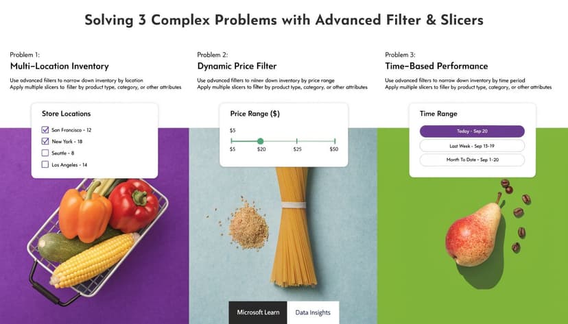
Solving 3 Complex Problems with Advanced Filter & Slicers

AutoFilter is great for everyday work, but it starts to feel cramped when your logic gets more specific. That's where Advanced Filter and Slicers earn their place.

Advanced Filter is more powerful than the standard Data > Filter workflow because it can evaluate multiple criteria across the full dataset and can also copy the filtered output to another range or worksheet, as explained in the Journal of Accountancy's overview of Advanced Filter. That “copy elsewhere” option is what turns it from a viewing tool into a reporting tool.

Problem 1 with AND logic

You need all rows where:

• Region = North
• Status = Open

AutoFilter can handle some layered filtering, but Advanced Filter is cleaner when you want a formal criteria setup you can reuse.

Create a small criteria area above or beside your data. Copy the exact column headers into that area. Under those headers, place:

• North under Region
• Open under Status

Put both conditions on the same row. That means Excel reads them as AND logic. The row must satisfy both conditions.

The criteria range must use copied headers from the source data. If the header text doesn't match, the filter often appears to “fail” when the real problem is setup.

Problem 2 with OR logic

Now the question changes. You want:

• Region = North
• or Region = West

A common challenge for many users arises with Advanced Filter, where OR logic goes on separate rows. So you'd copy the Region header once, then put North on one row and West on the next. Excel treats those lines as alternatives.

That same pattern can support more realistic business questions:

• open items or overdue items
• one product line or another
• one manager's accounts or another team's accounts

If you often search long drop-down lists while building these filters, this article on an Excel search box workflow can make selection faster in day-to-day files.

Problem 3 with extracting results for reporting

Sometimes you don't want to hide rows in the source sheet. You want a clean output somewhere else.

That's a strong use case for Advanced Filter. In the dialog box, choose Copy to another location, define the list range, define the criteria range, then choose the destination range. Excel pulls the matching records into that new area without disturbing the source table.

Here's the decision rule:

Need	Better tool
Quick inspection in place	AutoFilter
Multi-condition criteria with reusable setup	Advanced Filter
Clickable dashboard controls	Slicers

When slicers are the smarter choice

Slicers solve a different problem. They're visual. They're interactive. They're ideal when other people need to filter data without touching criteria ranges or formula logic.

If your data is in an Excel Table or PivotTable, you can insert Slicers and connect them to fields like Region, Category, or Owner. Instead of opening a drop-down, the user clicks a button-like control. For date-heavy PivotTables, Timelines provide the same idea with time-based filtering.

Use slicers when the workbook is meant to be used, not just analyzed once. They're a strong fit for dashboards, monthly review packs, and self-service reporting.

A Deep Dive into Excel's Dynamic FILTER() Function

The biggest shift in modern Excel filtering is that filtered results no longer have to stay inside a drop-down view. With FILTER(), the result can live in a separate part of the worksheet and update automatically.

Excel's FILTER function was added in Microsoft 365 and Excel 2021 and later, and it returns multiple matching rows dynamically rather than a single lookup result, as described in this FILTER function overview. That matters because the result can spill into adjacent cells and resize when the source data changes.

The syntax that matters

The structure is:

=FILTER(array, include, [if_empty])

Each part has a job:

• array is the range you want returned
• include is the test that tells Excel which rows to keep
• [if_empty] is optional text or a value to show if nothing matches

A simple example looks like this:

=FILTER(A2:D100, B2:B100="North", "No matches")

This formula returns rows from A2:D100 where the corresponding value in B2:B100 equals North. If no row matches, Excel shows No matches instead of an empty-result error.

That's a different mindset from AutoFilter. AutoFilter hides rows. FILTER() creates a live extracted result.

One condition and then two

Suppose your data has:

• Column A: Order ID
• Column B: Region
• Column C: Status
• Column D: Amount

To return only open records from the North region:

=FILTER(A2:D100, (B2:B100="North")*(C2:C100="Open"), "No matches")

The multiplication sign is the important part. In this context, it acts like AND. Both tests must be TRUE for a row to be included.

If you wanted North or West, you'd use addition:

=FILTER(A2:D100, (B2:B100="North")+(B2:B100="West"), "No matches")

That addition acts like OR. A row passes if either test is TRUE.

Key takeaway: In FILTER(), your logic lives inside the include argument. You're not stacking separate menu choices. You're building one Boolean test.

This guide to using the Excel FILTER function is helpful if you want more formula examples after you've practiced the basics.

Why formula-based filtering is so useful

A live formula result works well in dashboards, control sheets, and reporting tabs because it updates with the source data. You don't need to click a filter again every time a new row is added or a value changes.

That's why many analysts prefer FILTER() when they need:

• a report output that stays separate from raw data
• a clean feed for charts or summaries
• a repeatable model that someone else can audit by reading the formula

It also reduces a common workbook problem. With manual filters, the logic is often hidden in drop-down menus. With FILTER(), the logic is visible in the cell formula.

Where users get confused

Most mistakes come from one of three issues:

• Shape mismatch: The include range must align with the array being filtered
• Incorrect Boolean logic: Using the wrong operator changes the result
• Blocked spill range: The output needs enough empty cells to expand

When FILTER() works, it feels elegant. When it breaks, it usually breaks for one of those reasons.

A 5-Point Checklist for Troubleshooting Common Filter Issues

Filtering problems are frustrating because the worksheet often looks normal. The fix is usually simple, but only if you know what to check first.

The modern FILTER function returns live results using a single include argument built from Boolean logic, and complex conditions are created by chaining logical expressions. Exceljet also notes that spill errors or blanks can appear if the include array shape doesn't match the source array or if criteria are mis-specified in its FILTER function explanation.

1. The Filter button is greyed out

This often happens when the worksheet is protected or multiple sheets are grouped.

Check the sheet tabs first. If several tabs are selected, ungroup them. If the sheet is protected, remove protection if you have permission. Then try Data > Filter again.

2. New rows aren't included in the filter

This usually means your data is just a plain range, not a structured Excel Table.

Convert the range into a Table with Ctrl + T. Tables expand automatically as you add rows, which makes filters more reliable. If you stay with a normal range, you may need to reset the filter range manually.

3. FILTER() shows a #SPILL! error

The formula is trying to return multiple rows, but something is blocking the spill area.

Look below and to the right of the formula cell. Clear any existing values, spaces, or merged cells in that output area. Then recalculate. In many cases, the formula itself is fine.

If FILTER() should return several columns, every cell in the spill destination must be empty before Excel can place the result.

4. The results are blank or wrong

When FILTER() returns blanks or unexpected rows, inspect the logic before you inspect the data.

Use this quick check:

• For AND logic: Join conditions with *
• For OR logic: Join alternatives with +
• For matching ranges: Make sure the include range has the same height as the source array

If you're cleaning repeated records before filtering, this walkthrough on how to filter duplicates in Excel can help you fix the dataset before you troubleshoot the formula.

5. Blank and non-blank filtering behaves oddly

Blank cells in Excel can be real blanks, formulas returning empty text, or cells with hidden spaces. Those behave differently.

Try these checks:

Symptom	What to test
A “blank” row won't filter as blank	Check whether a formula returns ""
A non-blank row seems empty	Look for stray spaces
Some rows disappear unexpectedly	Check for inconsistent data types

Clean data beats clever filters. If the source values are inconsistent, the filter is only exposing the problem.

Beyond Manual Clicks with 1 AI-Powered Workflow

Manual filtering is fine when the request is simple. It gets clumsy when the request includes several steps at once, such as filtering by multiple conditions, copying the result to a new sheet, removing duplicates, and formatting the output.

That's where an AI agent inside Excel changes the workflow. Instead of deciding whether to use AutoFilter, Advanced Filter, or FILTER(), you describe the outcome in plain language. One example is Elyx AI's data cleaning workflow in Excel, which focuses on executing spreadsheet tasks rather than only explaining them.

A practical prompt might be:

Filter sales from the North region where status is Open, copy the result to a new sheet called Review List, and format the headers.

That request normally forces you to choose a method, prepare the output area, and check whether your ranges are structured correctly. With an AI workflow, the focus shifts from mechanics to intent.

This matters most when the workbook is messy or the task is repetitive. If you run the same kind of filtered extract every week, a natural-language workflow reduces setup work and lowers the chance of clicking the wrong menu or writing the wrong formula.

The skill still matters. You should understand what filtering is doing. But once you do, automation becomes a practical next step rather than a black box.

---

If you want Excel to execute filtering, cleaning, formatting, and reporting steps from a plain-English request, Elyx AI is built for that workflow inside Excel. It's useful when you already know the outcome you need and don't want to spend time on the intermediate clicks, formulas, or setup.