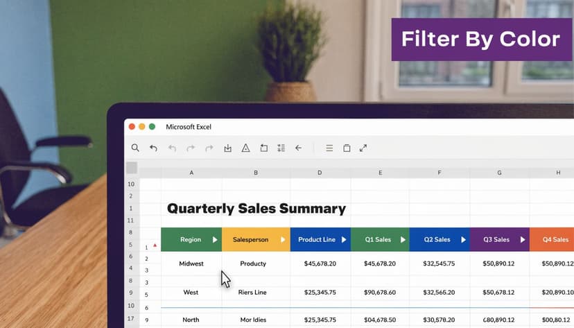
How to Filter by Color in Excel: 4 Essential Methods

You open a workbook from a colleague, and the logic lives in the colors. Red rows are urgent. Yellow rows need review. Green rows are done. The problem isn’t understanding the legend. The problem is acting on it without scanning row by row.

That’s where how to filter by color in Excel stops being a trick and starts being a workflow skill. If the sheet is already color-coded, Excel can turn that visual signal into an actionable list in a few clicks. If the sheet is messy, you can still work around most of the pain points once you know which method fits the job.

Why Mastering Color Filtering is a Superpower

A lot of business spreadsheets aren’t designed like databases. They’re designed by teams under pressure. Someone highlights exceptions in yellow, marks errors in red, and uses green to show approved items. That’s common in finance, project tracking, sales follow-up, and operations.

When you inherit a workbook like that, color filtering is often the fastest way to understand what matters first. You don’t need to rewrite formulas. You don’t need to build helper logic immediately. You use the structure that already exists.

Excel made this much easier starting in Excel 2007, when Filter by Color was introduced. Before that, users often needed VBA for similar behavior. One verified summary also notes that filtering challenges represented over 70% of Excel-related queries, and color-based filters resolved 45% of conditional data segmentation issues faster than formula-based methods, according to the cited source at this Excel color filtering walkthrough.

Where color filtering earns its keep

A few examples from real spreadsheet habits:

• Project plans where overdue tasks are filled red
• Expense reviews where questionable entries are highlighted yellow
• Sales trackers where high-priority accounts use custom fills
• QA logs where failed checks use red font instead of red fill

That last point matters. Excel treats cell color and font color as different filter types. Users mix them up all the time and assume the feature is broken, when they’re checking the wrong menu option.

Practical rule: If color carries business meaning in the sheet, learn to filter it before you start rewriting the file.

Color also works best when formatting is deliberate. If your workbook is inconsistent, fix the visual system first. A good starting point is this guide to formatting a worksheet in Excel, because cleaner formatting makes filtering more reliable.

Four methods matter in practice. The built-in AutoFilter is the fastest. Sort by Color helps when you need ranking instead of hiding rows. Tables and PivotTables change how filtering behaves. Automation comes last, when you’re repeating the same job every week.

Method 1 Your Quickest Path with AutoFilter

If you need a result in under a minute, use AutoFilter. It’s the built-in route one should typically start with.

Say you have a project tracker with these visual rules:

• Red fill = overdue
• Yellow fill = at risk
• Green fill = on track

You want to see only overdue tasks.

The fastest click path

1. Select any cell inside your data range.
2. Go to Data on the ribbon.
3. Click Filter.
4. Open the dropdown on the relevant column.
5. Choose Filter by Color.
6. Pick the fill color you want.

Excel hides all rows that don’t match that color. If your red rows are in the Status column, filtering there usually makes the most sense.

If your sheet isn’t structured well yet, it helps to clean the layout first. A practical companion step is learning how to organize data in Excel, because broken ranges and inconsistent headers are a common reason filters behave oddly.

Cell color and font color are not the same

This is one of the biggest mistakes I see.

If the cell background is colored, use Filter by Cell Color. If only the text itself is colored, use Filter by Font Color. Excel shows both when both exist in the selected column.

Here’s a simple approach:

What you see	What to choose
Yellow background in the cell	Filter by Cell Color
Red text on a white background	Filter by Font Color

If you choose the wrong one, Excel may show no matching result even though the sheet looks color-coded.

Filtering by color is only as good as the consistency of the column you filter on. If half the team colors the task name and the other half colors the due date, your result will be incomplete.

A good use case for AutoFilter

In a status sheet, AutoFilter is ideal when you need to answer questions like:

• Which tasks are overdue right now?
• Which rows were flagged for review?
• Which records were manually approved?

It’s fast because it doesn’t reorganize the data. It hides what you don’t need.

If you want a visual walkthrough, this short demo shows the menu sequence clearly:

What works and what doesn’t

Works well

• One clear status color per row
• A continuous data range with proper headers
• Manual fill colors or standard conditional formatting

Works poorly

• Blank rows splitting the range
• Merged cells
• Colors applied inconsistently across different columns
• Workbooks where users manually shade cells without any shared rule

If your goal is to isolate one color and work only on those records, AutoFilter is usually enough. If you need to keep every row visible but move priority items to the top, sorting is the better tool.

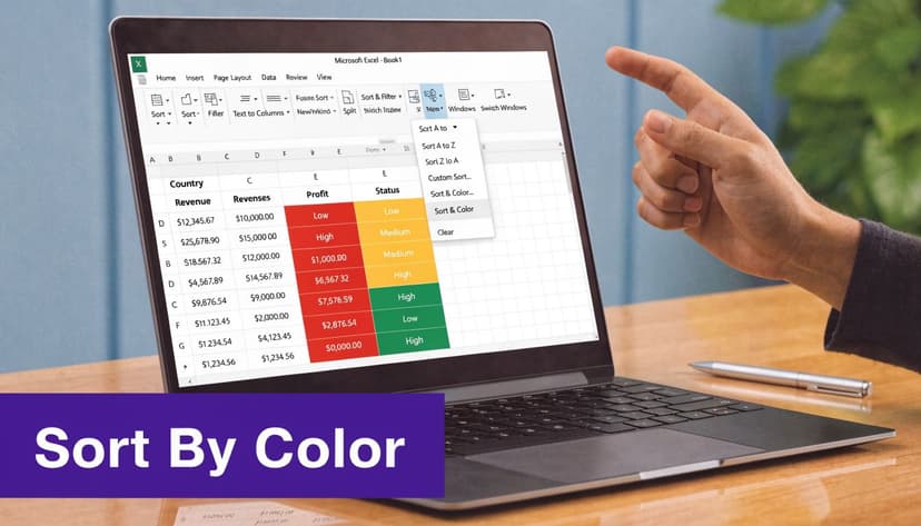
Method 2 Reordering Data with Sort by Color

Filtering and sorting look similar in conversation, but they solve different problems.

Filtering hides rows.
Sorting rearranges rows.

That difference matters when you’re building a working list for a meeting, a review queue, or a handoff. Sometimes you don’t want to hide anything. You want all the data visible, with the most important colors at the top.

When sorting is better than filtering

Take a sales pipeline where reps use fills like this:

• Green for strong opportunities
• Yellow for deals needing follow-up
• Red for stalled deals

A filter can show only red deals, but a sort gives you a ranked working view. You can put red first, yellow next, green last, and still keep the entire pipeline in front of you.

How to create a custom sort by color

Use this route:

1. Click inside the dataset.
2. Go to Data.
3. Click Sort.
4. In the Sort dialog, choose the column containing the colors.
5. Under Sort On, choose Cell Color or Font Color.
6. Under Order, pick the first color and choose whether it goes On Top or On Bottom.
7. Click Add Level to stack another color rule.
8. Repeat until your color order matches your priority order.

For example:

Sort level	Color	Position
1	Red	On Top
2	Yellow	On Top
3	Green	On Top

That creates a priority stack without removing lower-priority rows from view.

Why multi-level sorting is useful

Here, sorting becomes more practical than filtering. You can combine color with another rule.

For example:

• First sort by cell color
• Then sort by due date
• Then sort by owner

That gives you a real working queue. The urgent rows rise to the top, and within that group, Excel orders them in a way you can act on.

If you want to go deeper on formula-based sorting logic too, this reference on SORTBY in Excel is useful when you’re moving from manual sorting to dynamic formulas.

Use sorting when the color means priority. Use filtering when the color means selection.

Trade-offs to keep in mind

Sorting by color is great for review workflows, but it changes row order. That can be a problem if:

• Someone expects the original import order
• Your workbook references row positions manually
• You’re comparing before-and-after snapshots side by side

In those cases, create a helper column first or duplicate the sheet before sorting.

One more practical note. Multi-level color sorting is stronger than color filtering when your workbook contains several categories that all matter. You’re not forced into a single isolated view. You keep context, and context often matters more than a perfectly clean subset.

Method 3 Filtering Within Excel Tables and PivotTables

Color filtering behaves differently depending on whether your data is a plain range, an Excel Table, or a PivotTable. If you work in reporting environments, this difference matters more than the filter clicks themselves.

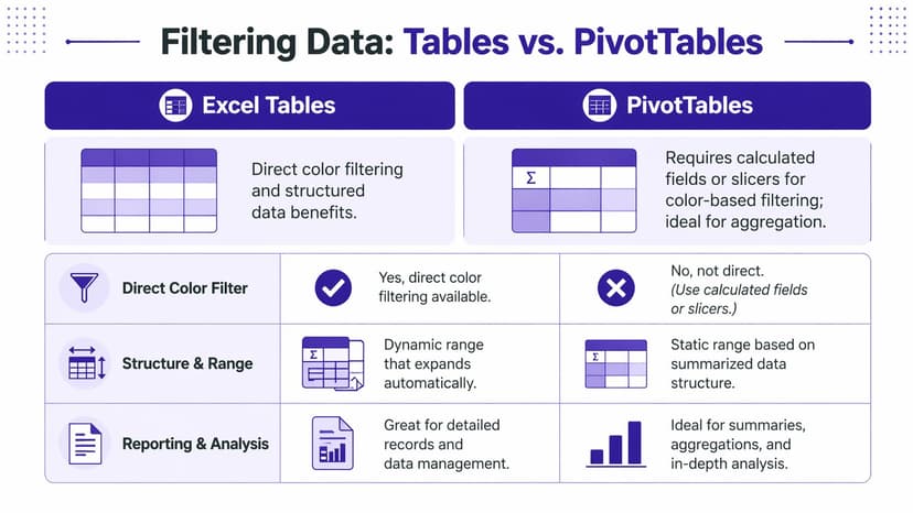
Tables are usually easier

An Excel Table is the most reliable place to use color filters in day-to-day work. Once your range is converted to a table, headers are locked in as filter controls, and the structure is more stable when rows are added.

That helps in messy business files, especially when data comes from imported reports, copied email tables, or even workflows involving extracting data from PDF into Excel, where structure often needs cleanup before analysis.

A quick comparison helps:

Feature	Excel Tables	PivotTables
Direct color filtering	Yes	Limited or indirect
Expands cleanly with new rows	Yes	Source-driven
Best for row-level review	Yes	No
Best for summaries and aggregation	Moderate	Yes

How to use color filters in a Table

If your range isn’t a table yet:

1. Select the range.
2. Press Ctrl + T.
3. Confirm that your table has headers.
4. Use the filter dropdown in the relevant column.
5. Choose Filter by Color.

This setup is better than filtering a loose range because tables handle expansion more gracefully. New rows added directly under the table become part of the structure automatically.

If you often analyze structured reports, this walkthrough on creating a PivotTable is a useful companion, because many teams move from table-level review to summarized reporting in the same workbook.

PivotTables are different for a reason

PivotTables summarize data. They aren’t designed primarily for row-level formatting logic.

That creates a practical limitation. If the color exists only in the source detail rows, a PivotTable doesn’t always expose that color in a clean, direct filtering workflow. You can sometimes filter a PivotTable by color in specific contexts, but it’s less dependable than filtering the underlying table.

What works better is this:

• Add a source column that stores the business meaning behind the color, such as Overdue, Review, or Approved
• Build the PivotTable from that explicit field
• Use normal PivotTable filters, slicers, or row labels on the text field

Don’t let color carry business logic alone inside a reporting model. Color is useful for scanning, but text fields are better for aggregation and reuse.

The practical decision

Choose Excel Tables when you need to inspect records, clean rows, and act on highlighted items.

Choose PivotTables when you need totals, grouped analysis, and summarized reporting. If color matters in the PivotTable stage, push that meaning into a proper column before you build the report.

That one design choice saves a lot of rework.

Method 4 Advanced Automation with VBA and AI

Manual color filters are fine until the task repeats every morning, across multiple sheets, with a follow-up action attached. At that point, the question is no longer "Can Excel filter by color?" It is "What is the fastest reliable way to finish the whole job?"

There are two practical options. Use VBA when the workbook is stable and the steps rarely change. Use an AI agent when the request includes several follow-on actions and the output changes from one run to the next.

A simple VBA script for filtering one color

For a fixed rule, VBA is still the cleanest tool. If column C always contains the highlighted cells you care about, this macro applies the filter in one step:

Sub FilterYellowRows()
    Dim rng As Range

    Set rng = ActiveSheet.Range("A1").CurrentRegion

    rng.AutoFilter Field:=3, Criteria1:=RGB(255, 255, 0), Operator:=xlFilterCellColor
End Sub

What this code does

• ActiveSheet.Range("A1").CurrentRegion captures the connected data block around cell A1
• Field:=3 applies the filter to the third column in that range
• RGB(255, 255, 0) targets yellow
• xlFilterCellColor tells Excel to filter by fill color

Two details matter in real work. CurrentRegion breaks if blank rows or columns split the dataset, and Field:=3 is positional, not tied to a header name. If someone inserts a column, the macro may still run and filter the wrong field.

That is why VBA works best in controlled workbooks.

If you build macros often, these Excel macro samples for common automation patterns are a useful starting point for adapting the script beyond a single color filter.

Where VBA starts to get expensive

The filter itself is rarely the full task. A manager usually wants a result package.

A typical request sounds more like this:

• filter the yellow rows
• copy them to a new sheet
• name the sheet High Priority
• group or summarize them by owner
• format the output for review

VBA can do all of that. I use it for repeatable reporting packs. The trade-off is maintenance time. Every extra step adds more code, more testing, and more ways for a workbook change to break the process.

Where an AI agent fits better

An autonomous AI agent such as ElyxAI handles a different kind of workload. Instead of writing each procedure, you define the outcome and let the agent carry out the sequence inside Excel.

A practical instruction looks like this:

Isolate all rows highlighted in yellow, copy them to a new sheet named High Priority, summarize them by owner, and add a chart.

That shifts the work from coding each action to specifying the result you want. It is especially useful when the request changes often, the workbook structure is mostly clean, and the post-filter steps take longer than the filter itself.

VBA versus AI in real work

Scenario	VBA	AI agent
One repeated color filter	Excellent	Good
Multi-step workflow after filtering	Possible, but slower to build	Faster to adjust
Requires coding knowledge	Yes	No
Mid-task changes from stakeholders	More rework	Easier to handle

The practical choice is simple. Use VBA for fixed, repeatable workflows where precision matters and the sheet structure is unlikely to change. Use an AI agent when the filtering task is only one step in a broader job and the final deliverable changes from request to request.

Both approaches still depend on disciplined workbook design. Clear headers, consistent fill colors, and uninterrupted ranges make automation far more dependable.

Troubleshooting 5 Common Color Filtering Problems

Color filters usually fail for predictable reasons. In practice, the problem is rarely the filter itself. It is usually a broken range, inconsistent formatting, or a sheet design that was never built for filtering in the first place. Microsoft’s filter by color guidance covers the core behavior, but these are the issues that slow people down in live workbooks.

1. The option is greyed out

Symptom: Filter by Color is unavailable.
Solution: Check the range first. Blank rows, blank columns, and partial selections often break the filter area. Reapply the filter to the full dataset, or convert the range to a table so Excel keeps the boundaries consistent.

2. Not all colors appear

Symptom: The dropdown shows fewer colors than expected.
Solution: Excel only lists colors found in the column you are filtering. If the fill color exists in another column, it will not appear in that menu. I also check for inconsistent shades here. Two cells can look similar and still count as different fills.

3. You need two or more colors at once

Symptom: One color filter is too limiting.
Solution: Color filtering works best for one visual category at a time. If you need several statuses together, add a helper column with text labels, or sort by color to group records before a second pass. That gives you more control than trying to force color into a job better handled by data values.

4. It behaves differently on desktop and online

Symptom: The menu or result changes across devices.
Solution: Test the workbook in the installed desktop version of Excel before you troubleshoot the data. Excel for the web can handle many filter tasks, but formatting behavior is still more dependable in current Microsoft 365 desktop builds.

5. Merged cells break the result

Symptom: Hidden rows and visible rows do not line up cleanly.
Solution: Unmerge them. Merged cells are one of the first things I remove when a client says filtering is unreliable, because they interfere with sorting, copying visible rows, and downstream automation.

If you only need to isolate a color once, stick with the built-in filter. If the task involves copying rows, creating a report sheet, summarizing results, and repeating the process every week, manual filtering stops being the bottleneck. The workflow around it does.

That is the point where the choice becomes practical. Use VBA when the workbook is stable and the steps are fixed. Use Elyx AI when the request changes from one file to the next and you want Excel to carry out the full sequence from a plain-language instruction, not just the filter step.