A Practical Guide to 3D Charts in Excel

Let's be honest: 3D charts in Excel get a bad rap. Many data professionals view them as flashy and confusing, and sometimes, they're right. But dismissing them entirely means leaving a powerful tool on the table. The key is knowing when and how to use them effectively. It’s not about making your data look cool for the sake of it; it's about adding a layer of understanding that a flat, 2D chart simply cannot provide.

This guide will show you how to solve a common business problem: visualizing complex data sets with multiple variables. By the end, you'll have a new skill—creating clear, purposeful 3D charts that reveal insights instead of hiding them.

When Do 3D Charts Actually Make Sense?

The real value of a 3D chart emerges when you need to compare data points across two different categories simultaneously. Move beyond a simple sales-over-time graph. Instead, picture yourself analyzing sales figures for different product lines across several geographic regions. This is where that third dimension adds real, tangible value, solving the problem of presenting three variables in a single view.

Making Sense of Multi-Variable Data

Imagine using a 3D clustered column chart for that sales scenario. Suddenly, you can see how each product is performing in every single region, all in one consolidated view. That depth axis (the Z-axis) makes it instantly clear which combinations are your winners, saving stakeholders from having to mentally stitch together insights from multiple charts or a dense table. In these moments, 3D shifts from a gimmick to an essential analytical tool.

This approach works wonders in other complex situations, too:

• Financial Modeling: Visualize how changes in interest rates and market volatility affect investment portfolio returns over several quarters.
• Scientific Data: A 3D chart is perfect for plotting experimental results where the outcome depends on two variables, like temperature and pressure.
• Market Analysis: Compare the market share of different competitors across various demographic segments.

The key to a great 3D chart is purpose. Always ask yourself: "Does this third dimension reveal a relationship that would otherwise be hidden?" If the answer is yes, you're on the right track.

The Impact of Geographic and Temporal Data

Excel's 3D Maps feature has also completely changed the game for analyzing data tied to a place or time. Think about mapping out market penetration by state or country. In my experience, presentations using 3D maps see 60-70% higher engagement than those with static 2D charts. Why? Because visually seeing those opportunities and risks on a map makes the data hit home for stakeholders.

To help you decide what's best for your specific data, here’s a quick guide.

Choosing Between 3D and 2D Charts

Scenario	Recommended Chart Type	Reasoning
Comparing sales across multiple product lines and regions.	3D Column or Bar Chart	Adds a necessary third dimension to show the relationship between all three variables at once.
Showing sales growth for a single product line over one year.	2D Line or Column Chart	A simple, clear comparison over a single variable (time). A 3D chart would add unnecessary clutter.
Plotting scientific results based on temperature and pressure.	3D Surface or Scatter Plot	Ideal for showing how a dependent variable changes in response to two independent variables.
Displaying budget allocation by department.	2D Pie or Donut Chart	Focuses on showing parts of a whole. Adding a third dimension would distort the proportions.
Mapping customer density across different zip codes.	3D Map	Provides geographic context that makes spatial patterns instantly recognizable.

This table isn't exhaustive, but it gives you a solid framework for thinking through your visualization choices.

Ultimately, the best chart depends on your dataset and the story you're trying to tell. While 3D charts won't be your go-to for every report, they are indispensable when you're working with multifaceted data. If you're looking to explore more advanced visualization options, our business intelligence software comparison is a great place to start.

Getting Your Hands Dirty: Your First 3D Chart in Excel

Alright, let's move from theory to action. This is where you really start to see how powerful (and sometimes tricky) 3D charts can be. We're going to walk through building three common types of 3D charts in Excel, each tied to a real-world business scenario you've probably encountered.

But first, a crucial piece of advice that will save you a ton of headaches: get your data organized before you even think about making a chart. A clean, logical table is the bedrock of a good visual. If your data is a mess, Excel will get confused, and you'll end up with a chart that makes no sense.

Comparing Sales with a 3D Clustered Column Chart

Let's kick things off with a 3D Clustered Column chart. This is best when you need to compare values across a couple of different categories. Say you're a sales manager and want to see how your regional teams stacked up against each other each quarter.

Your data table should be a simple grid:

• Rows: Your regions (e.g., North, South, East, West).
• Columns: Your time periods (e.g., Q1, Q2, Q3, Q4).
• Cells: The sales numbers for each region in the corresponding quarter.

Once your table is set up, select the entire range, including headers. Navigate to the Insert tab, find the Charts section, and click the Column or Bar Chart icon. Choose 3D Clustered Column. Excel will generate a chart with a group of columns for each region, making it easy to compare quarterly performance at a glance.

Quick tip from experience: Avoid selecting any "Total" row or column in your data. It skews the chart's scale, compressing the other data points and making them hard to read. Chart the raw data first; you can always add totals later as text or separate elements.

Slicing Up Budgets with a 3D Pie Chart

Next up, the 3D Pie chart. This is a classic for showing how a whole is divided, like a project budget. It’s great for getting a quick feel for proportions, but a word of caution: the 3D perspective can distort the visual size of the slices. We’ll cover how to mitigate this later.

The data setup is simple. You just need two columns:

1. Category: List the budget items (Marketing, R&D, Salaries, Operations).
2. Value: The dollar amount for each item.

Select your two columns, then navigate to Insert > Charts and find the Pie or Doughnut Chart button. Choose the 3D Pie option. Excel will instantly create a sliced-up pie where each piece represents a budget category, sized according to its share of the total.

Finding the Sweet Spot with a 3D Surface Chart

Now for a more advanced tool: the 3D Surface chart. Think of it as a topographical map for your data. It's perfect for finding the optimal combination of two different variables. For example, a marketing analyst might use it to see how ad spend and customer acquisition cost (CAC) combine to impact ROI.

The data structure here is very specific:

• Your top row contains one set of values (e.g., Marketing Spend increasing from left to right).
• Your first column contains the second set of values (e.g., CAC increasing from top to bottom).
• The cells in the middle are filled with the resulting metric—in our case, the ROI for each combination.

Select that whole grid of data. Go to Insert > Charts, click the icon that looks like a web (it's for Surface, Radar, or Stock Charts), and select 3D Surface. What you get is a flowing, colorful "landscape" of your data, complete with peaks and valleys that show you exactly where the sweet spots are.

If you're working with even more complex data that feels crammed, you might want to look into how to create a chart with a 2 Y-axis in Excel, which can help when you're comparing data on very different scales.

Making Your 3D Chart Actually Readable

So, you've clicked a button and Excel has given you a 3D chart. Great. But half the time, that default chart is a jumbled mess. This is where the real work begins. Moving beyond the default settings is what separates a confusing graphic from a professional, easy-to-understand visual.

The most powerful changes are hidden in the 'Format Chart Area' and, most importantly, the '3D Rotation' settings. These are the tools that let you control how people see your data, ensuring your main points stand out instead of getting lost.

Before we dive into tweaking, getting the chart on your worksheet is a simple three-part process.

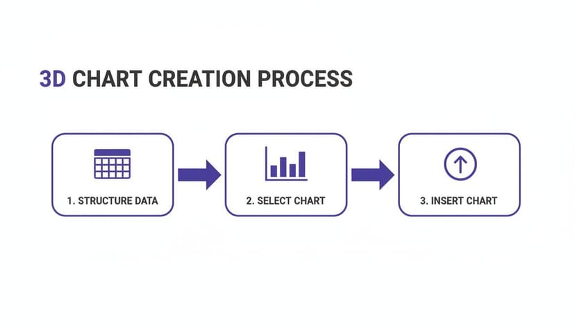
First, organize your data. Then, select the right chart type. Finally, insert it into your sheet. Now, we can start refining it.

Finding the Perfect Angle with 3D Rotation

The biggest problem with 3D charts is occlusion—when tall bars in the front completely hide shorter ones in the back, making your chart useless. The '3D Rotation' pane is your secret weapon against this.

To access it, right-click on your chart and choose "3D Rotation." You’ll see a few sliders to adjust.

• X Rotation: Tilts the chart forward and back. A small nudge can be all you need to reveal a data series that was hiding.
• Y Rotation: Spins the chart left or right. This is often the most effective tool for preventing columns from overlapping.
• Perspective: Controls the feeling of depth. Toning down the perspective a bit can make the elements in the back look less tiny and easier to compare.

Here's a practical tip: make small, one-degree-at-a-time adjustments. A tiny 5-degree spin on the Y-axis can be the difference between a cluttered mess and a clear picture.

Your goal is to find that sweet spot where every single data point is visible and the story your data is telling is obvious. You're trying to add a helpful sense of depth without distorting what the numbers actually mean.

Using Shadows and Lighting to Add Depth

Once you've set the viewing angle, you can add finishing touches to improve clarity. Go to the "Format Chart Area" pane and look under "Effects." You’ll find options for shadows and glows.

A light shadow behind your data bars or a subtle color on the chart's floor and walls can enhance the 3D effect. It helps guide the eye and makes the whole thing feel more polished and less like a default Excel graphic.

Excel offers a bunch of 3D chart options, from columns and bars to pies. When you take the time to customize them properly, you can boost how well people understand your report by an estimated 25-30%. You can learn more about 3D visualization capabilities on Microsoft's official site.

By getting the rotation just right and adding smart visual effects, you elevate a basic chart into an effective analytical tool. To get even more advanced, you can learn how to add a horizontal line to an Excel chart to call out important targets or averages.

Common 3D Chart Mistakes to Avoid

The "wow" factor of 3D charts in Excel can be tempting, but it can backfire spectacularly, turning your data into a confusing mess. The third dimension adds risks you just don't have with 2D charts, so you must be careful.

The most common problem is data occlusion—when taller bars or columns in the front completely block shorter ones in the back. Suddenly, your chart has blind spots, and your audience can't see the full story. It’s like taking a team photo with the tallest people standing in front; you’re not getting the complete picture.

The Problem of Perspective and Occlusion

To solve the issue of hidden data points, your go-to tools are rotation and transparency. A simple right-click on the chart gives you the "3D Rotation" option, where you can adjust the X and Y axis angles. Often, a small tweak is all you need to bring those hidden bars into view. Another trick is to make the front data series slightly transparent so you can see through them.

But be careful. Tweaking the rotation too much, especially with 3D pie charts, introduces a new problem: perspective distortion.

The slice closest to the viewer can look massive, while the one in the back seems tiny, even if they represent similar values. I've seen charts where a slice for 20% looked bigger than one for 25%—completely defeating the purpose of the chart.

Honestly? If you run into this with a pie chart, the best solution is to switch back to a simple 2D pie or a donut chart. It's more accurate.

Maintaining Data Integrity Above All

At the end of the day, a chart's job is to communicate information clearly and accurately. Before sharing any 3D chart, run through this quick mental checklist.

• Is every data point visible? If anything is hidden, you need to adjust the view or choose a different chart.
• Do the proportions look accurate? Double-check that the 3D effect isn't distorting the size of pie slices or columns.
• Does the third dimension add value? If it’s just adding visual clutter without providing new insight, stick with 2D. It’s almost always the safer, clearer choice.

Remember, a cool-looking chart that misleads people is worse than no chart at all. Many of these visualization headaches can also be avoided by ensuring your data is solid from the start. For a deeper dive, you might find these data cleaning best practices helpful. By sidestepping these common traps, you can create 3D charts that are both impressive and accurate.

Using ElyxAI to Automate Your 3D Chart Creation

Let’s be honest: building 3D charts in Excel by hand can be a real grind. Clicking through menus, highlighting data ranges, and tweaking formats eats up precious time. This manual effort pulls your focus away from what truly matters: analyzing the story your data is telling.

Artificial intelligence provides a solution to this problem. What if you could skip the manual steps? Imagine just telling Excel what you need, in plain English, and watching the perfect chart appear.

From Prompt to Polished Chart in Seconds

This is where an AI assistant like ElyxAI changes the game. It turns a tedious, multi-step process into a single, simple command. You just type what you want into a chat panel.

For example, you could write a prompt like:

"Create a 3D column chart showing Q3 sales broken down by product and region. Use our company's color palette and add data labels."

ElyxAI, leveraging the core theories behind Artificial Intelligence, understands this request. It finds the correct data on your worksheet and generates the exact 3D chart in Excel you asked for in moments. This isn't just a speed boost; it's about integrating best practices directly into the process. The AI handles formatting, labeling, and even finds a clear starting rotation to give you a professional-looking visual right away.

A Quick Look: Manual vs. AI-Powered Workflow

The efficiency gain is huge. Creating a detailed 3D chart by hand involves at least five to ten separate steps: selecting data, inserting the chart, choosing the type, formatting, rotating, and adding labels. Each click is another chance for error.

An automated, AI-powered workflow boils all of that down to a single action.

The Old Way (Manual)	The New Way (with ElyxAI)
1. Select the data range.	1. Write one clear instruction.
2. Go to Insert > Charts.
3. Choose the 3D chart type.
4. Right-click to format axes.
5. Adjust colors and styles.
6. Open 3D Rotation options.
7. Manually add data labels.

This shift gets you out of the weeds of Excel mechanics and lets you concentrate on what the chart is actually showing you. It’s a massive step forward for anyone looking to make their data analysis quicker and more insightful. If you want to see what else AI can do in your spreadsheets, check out our Excel AI assistant.

Answering Your Top Questions About 3D Charts

When you start working with 3D charts in Excel, a few common questions always seem to pop up. Here are the answers to the most frequent sticking points, which will help you solve problems before they start.

Can I Just Turn Any 2D Chart into 3D?

Not exactly. While Excel lets you easily add a third dimension to basic charts like column, bar, line, and pie charts (you can find these in the 'Change Chart Type' menu), the option isn't universal.

More specialized charts like Treemaps, Sunbursts, or Histograms are designed for 2D visualization and don't have 3D equivalents. For genuinely complex, multi-variable data, your best option is a 3D Surface chart. Just be aware that it requires a very specific X-Y-Z data layout to function properly.

How Can I Make My 3D Chart Easier to Read?

Readability is the biggest challenge with 3D charts in Excel. The single best tool to solve this is the '3D Rotation' feature. Right-click your chart and select '3D Rotation' to bring up the controls.

My advice: make small, careful adjustments to the X and Y rotation values. The goal is to find an angle where taller columns don't block smaller ones behind them—a problem called occlusion. It also helps to reduce the 'Perspective' setting to minimize distortion. For maximum clarity, add data labels directly to your chart. For example, if your chart values are in column C, you can use a formula to check for small values that might be hard to see:
=IF(C2<500, "Label: " & C2, C2)
This formula would add a "Label:" prefix to any value under 500, drawing attention to smaller data points.

A well-rotated chart should make every data point visible. The goal is to enhance understanding with depth, not to create a visual puzzle that obscures the information.

What's the Difference Between a 3D Chart and 3D Maps?

Although they sound related, they are different tools for different problems.

A standard 3D chart, like a 3D column chart, adds a depth axis to regular data categories. It's for comparing standard numerical data, but with an extra visual dimension.

On the other hand, 3D Maps is a specialized tool built for one purpose: plotting geographic data. If your spreadsheet has columns for countries, states, cities, or zip codes, this is the tool you need. It turns your data into an interactive 3D globe, perfect for spotting regional sales trends or mapping out a supply chain. Think of it as a geo-spatial analysis tool, while a regular 3D chart is a general-purpose visual.

---

Ready to stop wrestling with manual chart creation and get straight to the insights? Elyx.AI is an AI agent that builds complete, professionally formatted charts from a single instruction. Describe what you need, and watch as it performs the work for you, directly in your spreadsheet. Start your free 7-day trial today and see how much time you can save.