How to Compare Two Excel Sheets with Simple Proven Methods

Comparing two Excel sheets is a fundamental task, but the method you choose can make all the difference. You can opt for a quick visual check with Conditional Formatting, perform a detailed lookup with formulas like VLOOKUP or INDEX-MATCH, or leverage the industrial-strength capabilities of Power Query. The right tool depends on your data's complexity and volume. Regardless of the path, the objective remains the same: ensuring data integrity and eliminating costly manual errors. This guide will walk you through practical, actionable methods to master this essential skill.

Why Comparing Excel Sheets Is a Critical Skill

Comparing spreadsheets is not just a technical task; it's a foundational skill for anyone working with data. Relying on manual scanning is not only slow—it's a direct path to inaccurate results. A single missed update in a financial report can skew budget forecasts, while an overlooked change in an inventory list could lead to stockouts during a critical sales period. These are the real-world problems that a systematic comparison process solves.

The Impact on Daily Business Operations

Consider a typical month-end close. Accounting teams often manage multiple versions of reports, making it easy for small errors to slip into the final numbers. An analyst proficient in comparing Excel sheets can instantly spot discrepancies, ensuring the final report is accurate and reliable.

This skill is crucial across various departments:

• Auditing: Auditors routinely compare asset lists from one quarter to the next to track acquisitions and disposals with precision.
• Marketing: A team might compare a new lead list against their existing CRM data to identify and tag new subscribers for a targeted welcome campaign.
• Human Resources: An HR specialist needs to reconcile payroll records from different systems to confirm that all salary adjustments were processed correctly.

The core benefit is shifting from assumption to certainty. Instead of hoping your data is correct, you implement a repeatable process to prove it. This confidence is invaluable when your decisions impact the bottom line.

Moving Beyond Manual Checks

The primary drawbacks of manual checks are human error and excessive time consumption. It is easy to miss a transposed number or a minor typo in a large dataset. Mastering Excel's comparison tools transforms this process.

By adopting a structured method, you eliminate tedious and unreliable visual scans. You create a system that is not only faster but also fully auditable. This allows you to focus your energy on analyzing what the data differences mean for the business, rather than just finding them. This process, known as data reconciliation, is a cornerstone of effective data management. To learn more about its principles, you can explore this resource on what data reconciliation is.

Ultimately, mastering sheet comparison elevates your role from a simple Excel user to a data professional who can confidently stand behind their numbers.

Getting Started: Formulas and Formatting

Before exploring advanced add-ins or external tools, it’s essential to master the powerful features already built into Excel. Formulas and visual tools are the workhorses for most comparison tasks. A solid grasp of these fundamentals will prepare you for nearly any data comparison challenge, from a quick spot-check to a detailed analysis.

The most direct method for visualizing differences is Conditional Formatting. It acts like a magic wand, making discrepancies stand out visually. Instead of manually scanning rows, you can instruct Excel to automatically color-code unique values, duplicates, or any cells that don't match. This is the ideal method for getting a quick, high-level overview of your data.

See the Differences Instantly with Conditional Formatting

Imagine you have two lists of product IDs—one from last month's inventory (Sheet1) and one from this month (Sheet2). Your goal is to identify new products. Simply highlight the product ID column in Sheet2, navigate to the Home tab, click Conditional Formatting, and create a new rule using a formula.

This immediate visual feedback is a significant time-saver. While powerful for spotting differences, manual methods like this can be slow and introduce risk. Manually comparing two sheets with just 10,000 rows can take 3 to 5 hours, with a potential error rate as high as 5%.

While conditional formatting excels at highlighting differences, it doesn't explain what those differences are or pull in related data. For that, we need to leverage Excel's formulas. For a complete tutorial on this feature, refer to our guide on how to use Conditional Formatting in Excel.

Digging Deeper with Formulas

When you need more than a highlighted cell, formulas are the answer. They can verify if a value from one sheet exists on another, flag mismatches, and retrieve related data to provide a complete picture. The three most effective formulas for this are VLOOKUP, INDEX-MATCH, and COUNTIF.

The key is to know which formula to use for a given task.

• COUNTIF: Ideal for a simple "yes or no" check. It answers the question, "Does this value from Sheet1 exist anywhere in this column on Sheet2?"
• VLOOKUP: The classic choice for direct lookups. It finds a value in the first column of a table and returns a corresponding value from another column in the same row.
• INDEX-MATCH: A flexible and powerful alternative. It overcomes VLOOKUP's limitations by allowing you to look up a value in any column and return data from any other column, regardless of its position.

A common mistake is using a complex INDEX-MATCH when a simple COUNTIF would suffice. Always start with the simplest tool that meets your needs. This keeps your workbook efficient and your logic easy to understand.

Real-World Example: Finding New Hires

Let's apply this to a practical scenario. You have a master employee roster (MasterList) and a list of this month's new hires (NewHires). You need to confirm that individuals on the NewHires list are not already in the master file, which could happen due to rehires or data entry errors.

In your NewHires sheet, add a new column named "Verification." In the first cell of this column, enter the following COUNTIF formula:

=COUNTIF(MasterList!$A:$A, A2)

Here’s a breakdown of the formula:

1. MasterList!$A:$A: This tells Excel to search the entire column A on the MasterList sheet, where your master employee IDs are stored. The $ symbols lock the reference, ensuring it remains fixed as you copy the formula down.
2. A2: This refers to the employee ID in the current row of your NewHires sheet.

Drag this formula down the "Verification" column. It will return a 1 if the employee ID is found on the master list and a 0 if it is not. You can then filter for the zeros to get a clean, accurate list of new employees. A task that could have taken hours manually is now completed in seconds.

When formulas and conditional formatting aren't enough, Excel offers more specialized tools designed for complex comparison jobs involving massive datasets or requiring forensic levels of detail. These professional-grade options ensure you can compare two Excel sheets without any margin for error.

Choosing Your Excel Comparison Method

Before diving into advanced techniques, it's useful to understand your options. The best method depends on your objective, data size, and time constraints.

This table will help you select the right tool for your specific task.

Method	Best For	Pros	Cons
VLOOKUP/INDEX-MATCH	Finding matching or missing records based on a unique ID. Great for cross-referencing lists.	Quick to implement for simple lookups; flexible.	Can be slow on large datasets; prone to errors if not set up correctly.
Conditional Formatting	Quick visual checks to spot differences or duplicates directly on your sheets.	Instant visual feedback; easy for anyone to understand.	Not great for summarizing findings; can be slow on very large ranges.
Inquire (Spreadsheet Compare)	Deep, structural audits of workbooks to find changes in formulas, formatting, or even VBA code.	Extremely thorough and detailed; catches things manual checks miss.	Only available in specific versions of Excel (Microsoft 365 Apps for enterprise).
Power Query (Merge Queries)	Comparing massive datasets that would crash standard Excel functions.	Incredibly powerful and efficient for millions of rows; handles complex joins easily.	Steeper learning curve; overkill for simple, small-scale comparisons.
VBA/Macros	Automating custom, repetitive comparison tasks that you perform regularly.	Fully customizable and automated; can be tailored to exact needs.	Requires programming knowledge; can be complex to write and debug.

Ultimately, the best method is the one that fits your specific challenge. For a simple list check, a formula is perfect. For a multi-million row database comparison, Power Query is your only real option.

Uncovering Every Change with Spreadsheet Compare

Have you ever inherited a complex financial model and needed to identify changes between versions? Or had to audit a workbook for compliance? For these tasks, the Inquire add-in is the solution. It is a powerful tool available in certain enterprise versions of Excel.

The key feature of this add-in is Spreadsheet Compare. This tool goes beyond comparing cell values; it performs a forensic analysis of your entire workbook, meticulously flagging differences that are nearly impossible to spot manually.

Spreadsheet Compare can pinpoint discrepancies in:

• Formulas: Detects if a SUM was accidentally changed to an AVERAGE.
• Cell Formatting: Flags subtle changes in number formats that can alter data interpretation.
• VBA Code: Shows if a macro was modified, potentially changing an entire automated process.
• Hidden Rows or Columns: Uncovers data that may have been hidden intentionally or accidentally.

This level of detailed analysis is invaluable in fields like finance and auditing, turning hours of manual review into a minutes-long task. To see it in action, check out this Microsoft Mechanics video on automating Excel comparisons.

To use it, you first need to enable the Inquire add-in from Excel's Options menu (under Add-ins > COM Add-ins). Once enabled, a new "Inquire" tab will appear on your ribbon, providing direct access to Spreadsheet Compare.

This simple flowchart can help you decide between a quick visual check with Conditional Formatting or a more robust formula-based approach like VLOOKUP.

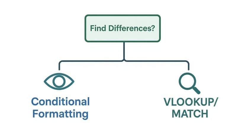
As shown, Conditional Formatting is best for a quick visual highlight. However, when you need to retrieve data from one sheet to another based on a match, a lookup formula is the more powerful choice.

Handling Large Datasets with Power Query

What if your data is massive, spanning hundreds of thousands or even millions of rows? Attempting a VLOOKUP on such a dataset will likely cause Excel to freeze and crash. This is where Power Query excels. It's Excel's data-shaping and analysis engine, designed to handle vast amounts of information efficiently without slowing down your computer.

The key feature for this task is Merge Queries. This allows you to join two tables based on a common column (like an 'Order ID' or 'Product SKU'), similar to a database join. You start by loading both sheets into the Power Query editor, then use "Merge Queries" to specify the columns to match.

The real power of Power Query lies in its "Join Kinds." You are not just finding matches; you are instructing Excel on how to compare the lists, giving you complete control over the output.

For comparison tasks, these three join types are particularly useful:

• Inner Join: Shows only the rows that exist in both sheets, perfect for finding common records.
• Left Anti Join: A powerful option for finding discrepancies. It returns all rows from the first sheet that do not have a match in the second, cleanly identifying what's missing.
• Full Outer Join: Combines all rows from both sheets, aligning matches and showing unique items from each. This provides a complete overview of matches and differences in one table.

After Power Query processes the data, you load only the results—the differences you need—back into a new worksheet. Your original large files remain untouched, and your workbook stays responsive. Mastering this skill is essential for reliably comparing two Excel sheets at scale.

Automating Comparisons with VBA and AI

When you have pushed Excel's built-in tools to their limits, automation is the next step. If you perform the same complex comparison regularly, creating a system to do it for you can save countless hours and virtually eliminate human error. This is where you transition from simply working in Excel to making Excel work for you.

Building Your Own Comparison Tool with VBA

Visual Basic for Applications (VBA) is Excel's built-in programming language, allowing you to create custom macros. A macro is a sequence of actions that you can execute with a single click. Instead of manually applying formulas or formatting rules each time, you can write a script that performs the task perfectly, tailored to your specific needs.

For example, if you need to compare two large inventory sheets ("Sheet1" and "Sheet2") daily, a VBA macro can iterate through each cell in a specified range on the first sheet, compare its value against the corresponding cell on the second sheet, and highlight any differences in red.

Here is a simple VBA script for this task:

Sub HighlightDifferences()
    Dim ws1 As Worksheet, ws2 As Worksheet
    Dim range1 As Range, range2 As Range
    Dim cell As Range

    ' Set your two worksheets by name
    Set ws1 = ThisWorkbook.Sheets("Sheet1")
    Set ws2 = ThisWorkbook.Sheets("Sheet2")

    ' Define the range to compare in Sheet1
    Set range1 = ws1.Range("A1:E100")

    ' Loop through each cell in the defined range
    For Each cell In range1
        ' Check if the cell value in Sheet1 is different from Sheet2
        If cell.Value <> ws2.Range(cell.Address).Value Then
            ' If different, color the cell in Sheet1 red
            cell.Interior.Color = vbRed
        End If
    Next cell

    MsgBox "Comparison complete. Differences are highlighted in red."
End Sub

The true power of VBA lies in its adaptability. You can modify scripts to handle dynamic ranges, compare based on specific criteria, or even generate a summary report of all discrepancies. It's a one-time investment that provides ongoing returns in productivity.

To use this script, open the VBA editor (Alt + F11), paste the code into a new module, and run the macro. This small step into coding can yield a significant improvement in efficiency. For more on building automated workflows, our article on how to automate Excel reports is an excellent resource.

The Rise of AI in Excel Comparisons

While VBA is powerful, it comes with a learning curve. The future of Excel automation is more intuitive, driven by conversational AI. New tools, including our own Elyx.AI, are transforming the user experience. Now, you can perform complex comparisons simply by describing your requirements in plain English.

Instead of writing code or remembering complex formula syntax, you can ask an AI assistant to perform the task for you. This makes advanced data analysis accessible to everyone, regardless of their technical expertise. For an overview of this technology, a practical guide to AI automation offers valuable insights.

Using Natural Language for Complex Tasks

Revisiting our earlier examples, instead of manually constructing a Power Query merge or a VBA script, you could give an AI assistant a simple prompt:

• "Find all rows in Sheet1 that don't exist in Sheet2, using 'Order ID' as the key."
• "Compare column B in 'January Sales' to column B in 'February Sales' and highlight any values that decreased."
• "Create a new sheet summarizing the differences between 'Old_Inventory' and 'New_Inventory'."

The AI interprets your request, executes the appropriate process behind the scenes, and delivers the result. It can format cells, generate a summary table, or even show you the formula it used, providing a learning opportunity. This represents a fundamental shift from manually performing tasks to directing outcomes.

This AI-powered approach offers several key advantages:

• Rapid Prototyping: Test different comparison methods in seconds without committing to a complex setup.
• Ad-Hoc Analysis: Get quick answers to one-off questions without disrupting your workflow.
• Continuous Learning: Improve your Excel skills by observing the formulas and methods the AI employs.

By integrating AI directly into the spreadsheet, the barrier between your question and your answer disappears. The entire process of how to compare two Excel sheets becomes faster, more accurate, and refreshingly straightforward.

Best Practices for Flawless Data Comparison

Knowing the different methods to compare two Excel sheets is only half the battle. Ensuring the accuracy of your results depends on good data hygiene and disciplined processes. The most effective analysts understand that preparation is crucial for success. The following tips serve as a pre-comparison checklist to ensure your foundation is solid.

Standardize and Clean Your Data First

Before you begin any comparison, you must clean and standardize your data. Inconsistent formatting is a common cause of failed comparisons and inaccurate results.

Develop a habit of addressing these issues first:

• Hidden Spaces: Use the =TRIM() function on key columns to remove leading or trailing spaces. "Product A " will not match "Product A" without this step.
• Number and Date Formats: Ensure numbers are stored as numbers and dates use a consistent format across both sheets. To Excel, "10/05/2024" and "Oct 5, 2024" are different values.
• Case Sensitivity: Use the =UPPER() or =LOWER() function to standardize text, preventing mismatches between "Apple" and "apple."

A unique identifier is essential for a reliable comparison. This is a column where every value is distinct, such as an Employee ID or an Order Number. Without a dependable key, your comparison will be based on guesswork.

Document Your Process and Handle Large Files

When working with large datasets, Excel can become slow. To improve performance, avoid using entire column references like A:A in your formulas. Instead, use specific ranges like $A$1:$A$50000 or, even better, structured Excel Tables to reduce calculation time significantly.

Documenting your methodology is equally important. Whether you used Power Query, a VBA script, or a series of formulas, leave comments or maintain a log explaining your logic. This makes your work auditable and understandable for colleagues—or for yourself in the future. It is a critical step in building trust in your results.

Fine-Tune Your Comparison Approach

Different comparison methods have varying performance characteristics. For many tasks, simple formulas like VLOOKUP or conditional formatting are highly effective. For example, businesses comparing product inventories have found that a VLOOKUP-based process can reduce mismatches by 40% compared to manual visual checks.

As you incorporate modern tools into your workflow, data security must remain a priority. When exploring AI-powered comparisons, it is critical to ensure a GDPR compliant AI integration from the start. This protects sensitive information and ensures your methods align with current data privacy standards.

Got Questions? I've Got Answers

When you start comparing Excel sheets, you will likely encounter some challenges. Here are answers to some of the most common questions, based on years of practical experience.

How Can I Quickly See What's Different in Just One Column?

The fastest way to identify differences in a single column is by combining COUNTIF with Conditional Formatting. This technique provides immediate visual feedback by highlighting every cell that is unique to one list.

Suppose you have a list of product IDs in column A of "Sheet1" and another list in column A of "Sheet2." You want to see which IDs from Sheet1 are missing from Sheet2.

Follow these steps:

1. Highlight the column of product IDs on Sheet1 (e.g., A2:A500).
2. Go to the Home tab, click Conditional Formatting, and select New Rule.
3. Choose the option "Use a formula to determine which cells to format."
4. In the formula box, enter: =COUNTIF(Sheet2!$A:$A, A2)=0

This formula checks each ID in your selected range (starting with A2) and counts its occurrences in column A of Sheet2. If the count is zero, it means the ID is missing from the second sheet, and Excel will apply your chosen formatting, making discrepancies instantly visible.

What's the Best Way to Compare Massive Files Without Excel Crashing?

For datasets exceeding 100,000 rows, avoid using worksheet formulas. Power Query is the ideal solution. It is designed to handle large volumes of data efficiently because it processes the data outside the main Excel grid, preventing freezes and crashes.

The key feature to use is Merge Queries.

• First, load both of your large tables into the Power Query editor.
• Next, use "Merge Queries" to link them using a unique identifier, such as an order number or employee ID.
• To find missing records, perform an Anti Join (either Left Anti or Right Anti). This join type is specifically designed to show only the rows from one table that have no corresponding match in the other.

This method is incredibly efficient. Instead of forcing Excel to perform calculations on millions of rows, you load only the final results—the actual differences—back into a new sheet.

I once needed to compare two sales reports, each with over a million rows. A VLOOKUP would have been unfeasible. Using Power Query's Left Anti Join, I isolated the 5,000 unmatched records in under two minutes.

Can I Compare Two Columns and Grab Data from a Third?

Yes, this is a common data validation task and the perfect application for VLOOKUP or the more versatile INDEX and MATCH combination. While VLOOKUP is more straightforward for beginners, INDEX-MATCH is often preferred for its flexibility—the lookup column does not need to be the first one in the table.

Imagine you need to verify salaries. You have an Employee ID in column A on both sheets, and the updated salary is in column D of "Sheet2." To pull that salary into "Sheet1" for comparison, you would place this formula next to the first employee ID:

=INDEX(Sheet2!D:D, MATCH(A2, Sheet2!A:A, 0))

Here's how it works:

• MATCH(A2, Sheet2!A:A, 0) finds the employee ID from Sheet1 (cell A2) in the ID column of Sheet2 and returns its row number.
• INDEX(Sheet2!D:D, ...) takes that row number and retrieves the value from column D (the salary) in Sheet2.

If an ID from Sheet1 does not exist on Sheet2, the formula returns an #N/A error, which is useful for instantly flagging missing records. This is a go-to technique for building a detailed comparison report.

---

Ready to stop wrestling with complex formulas and start getting answers in seconds? Elyx.AI integrates directly into your Excel workflow, allowing you to compare, clean, and analyze your data using simple, natural language. Ask questions, generate formulas, and build reports without ever leaving your spreadsheet. Transform your Excel experience by visiting the official Elyx.AI website to learn more.