How to Calculate Gross Margin in Excel The Right Way

Calculating gross margin is a fundamental skill for understanding a business's financial health. The formula itself is straightforward: (Revenue – Cost of Goods Sold) / Revenue. But mastering its application in Excel is what turns raw data into actionable business intelligence.

This guide will show you how to calculate gross margin in Excel, from basic formulas to advanced analysis using Pivot Tables and AI. By the end, you'll have a practical skill set to efficiently measure your company's core profitability.

Why Gross Margin Is a Vital Sign for Your Business

Before we jump into Excel formulas, let's establish why gross margin is so critical. Think of it as a direct measure of your business's core operational efficiency. It answers a simple but profound question: for every dollar of revenue, how many cents are left after paying for the goods sold?

This metric is a direct reflection of your production efficiency and pricing strategy. A healthy gross margin ensures you have enough cash to cover all other operating expenses, such as marketing, R&D, and administrative salaries, while still generating a profit.

The Building Blocks of Gross Margin

The calculation relies on two key financial data points:

• Revenue: This is the total income from sales. For an accurate calculation, you should always use net revenue, which is your total sales minus any customer returns or discounts.
• Cost of Goods Sold (COGS): These are the direct costs incurred in producing the goods or services you sell. This includes raw materials and direct labor. It does not include indirect costs like marketing salaries or office rent.

Let's use a practical example. Imagine you're a financial analyst at a Software-as-a-Service (SaaS) company. Your task is to evaluate the profitability of a new product.

Your sales data shows $1 million in software license revenue. The direct costs associated with delivering this software (like server hosting and dedicated developer support) amount to $200,000. Using the formula, your gross margin would be 80%. This is a strong result, aligning well with the typical 75%-85% benchmark for the SaaS industry.

A higher gross margin means you have more money to reinvest into growth, pay for operating expenses like marketing and R&D, and ultimately, generate net profit. It’s the foundational metric that shows if your business model is sustainable at its most basic level.

Understanding this metric is a key part of many financial analysis techniques. For any business, accurately tracking COGS and revenue is non-negotiable. If you're ever unsure about your numbers, it can be a good idea to work with professional accounting services to ensure everything is spot-on.

Getting these fundamentals right makes the practical Excel steps we're about to cover much more powerful.

Calculating Gross Margin Manually in Excel

Now, let's move from theory to practice within Excel. Manually calculating gross margin is a fundamental skill that provides a granular view of your product profitability. All you need is a clean data setup and two simple formulas.

First, ensure your spreadsheet is organized. A common setup includes product names in column A, Net Revenue in column B, and your Cost of Goods Sold (COGS) in column C.

Building the Gross Profit Formula

The first step is to calculate Gross Profit—the raw dollar amount left after subtracting COGS from revenue.

In cell D2, next to your first row of data, type the following formula:

=B2-C2

Let's break down this Excel formula:

• The = sign initiates the formula, telling Excel to perform a calculation.
• B2 is a cell reference pointing to the Net Revenue for the first product.
• - is the subtraction operator.
• C2 is a cell reference pointing to the COGS for the same product.

Press Enter. If the revenue in B2 was $500 and COGS in C2 was $200, cell D2 will now display $300.

Calculating the Gross Margin Percentage

Gross Profit is useful, but Gross Margin percentage is the key performance indicator (KPI) that shows profitability relative to revenue.

In the next column, cell E2, enter this formula:

=(B2-C2)/B2

This formula executes in two steps due to the parentheses (following the order of operations):

1. It first calculates the Gross Profit (B2-C2).
2. It then divides that result by the Net Revenue (B2).

After pressing Enter, Excel will likely display the result as a decimal, such as 0.6.

Pro Tip: To make this decimal more readable, format it as a percentage. Select cell E2 (or the entire E column), navigate to the 'Home' tab on the Excel ribbon, and click the percent style (%) button. The value 0.6 will instantly convert to 60%.

For a deeper dive into this functionality, our guide on how to calculate percentage in Excel provides more examples and tips.

Once you have the formulas in D2 and E2, you don't need to retype them for every row. Click on one of the cells and locate the small square in the bottom-right corner—this is the fill handle. Double-click it, and Excel will automatically copy the formulas down for all your data, saving you significant time.

Uncovering Deeper Insights with Pivot Tables

Calculating gross margin row-by-row is useful for a granular view, but the real strategic power comes from aggregating this data. When you need to understand profitability across product categories, sales regions, or time periods, a Pivot Table in Excel is the perfect tool.

A Pivot Table allows you to create a dynamic summary of your data without adding extra formula columns to your source sheet. This keeps your original data clean and enables you to slice and dice your gross margin analysis on the fly.

Creating a Calculated Field for Gross Margin

The key to performing calculations within a Pivot Table is the Calculated Field feature. This lets you define a new formula that operates on the summarized data, updating automatically as you rearrange your report.

Here’s how to create a Calculated Field for Gross Margin, assuming your source data has 'Revenue' and 'COGS' columns:

1. Select your data range and go to Insert > PivotTable. Click OK to create it on a new worksheet.
2. Click anywhere inside your new Pivot Table to activate the PivotTable Analyze tab in the ribbon.
3. Navigate to Fields, Items, & Sets and select Calculated Field.
4. In the 'Name' box, enter a descriptive name like "Gross Margin".
5. In the 'Formula' box, type the gross margin formula using your field names: = ('Revenue' - 'COGS') / 'Revenue'
6. Click OK. Your new "Gross Margin" field will appear in the PivotTable Fields list.

Now you can use this field like any other. For instance, drag 'Product Category' to the Rows area and your new 'Gross Margin' field to the Values area. The Pivot Table will automatically calculate the overall gross margin for each category.

A well-structured Pivot Table does more than just report numbers; it tells a story about your business. It can instantly highlight that your 'Electronics' category has a 75% margin while 'Accessories' are only at 35%, guiding your inventory and marketing strategy without any extra manual work.

This approach gives you incredible flexibility. In seconds, you can pivot your view to see which sales region is the most profitable or which product line is dragging down your average. For a complete walkthrough, check out our Excel Pivot Table tutorial.

Using AI to Automate Your Gross Margin Analysis

While manual calculations and Pivot Tables are powerful, they can be time-consuming and prone to human error. This is where AI tools integrated with Excel are changing the game, allowing you to move from tedious data preparation to actionable insights with a single command.

Imagine receiving a messy sales export with extra spaces, inconsistent number formats, and blank cells. Before you can even begin your analysis, you face a data cleaning chore. An AI agent like Elyx.AI automates this entire workflow, from data cleansing to final analysis.

From Multiple Steps to a Single Prompt

Instead of manually adding columns, writing formulas, and configuring a Pivot Table, you can simply describe your desired outcome in plain English. This allows you to focus on strategic interpretation rather than the mechanics of Excel.

For example, with your raw sales data selected, you could give an AI assistant a prompt like this:

"Calculate the gross margin for each row using the 'Revenue' and 'COGS' columns. Then, create a pivot table that shows the average gross margin by 'Region'. Finally, highlight any products with a margin below 20% in red."

In seconds, an AI agent can execute these instructions. It will clean the data, insert the correct formula, build the Pivot Table, and apply conditional formatting. This not only saves time but also reduces the risk of formula errors that could compromise your entire analysis. The real power of integrating AI in Excel lies in its ability to handle these multi-step workflows autonomously.

For a finance team, mastering this kind of workflow means you can spot profitability issues almost in real-time. While many small businesses aim for a 7-10% margin, this level of automation helps you dig deeper and push for better performance, turning your spreadsheets into true profit-driving tools. For a deeper dive into industry standards, check out these gross margin benchmarks on grossmargin.co.uk.

Visualizing Your Path to Profit

The goal of automation is to streamline the path from raw data to actionable insight. This workflow shows how a Pivot Table—whether built manually or with AI—transforms a simple spreadsheet into a source of strategic intelligence.

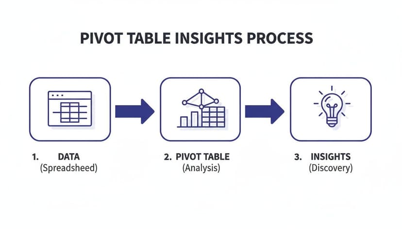
As you can see, it’s a clear path: good, clean data is the foundation for a dynamic Pivot Table, which then gives you the insights you need to make smarter business decisions.

Manual Excel vs Elyx AI Workflow

The following table compares the traditional Excel process with an AI-powered approach for a typical gross margin analysis.

Task	Manual Excel Steps	Elyx AI Prompt
Data Cleaning	1. Use TRIM for spaces. 2. Find & replace errors. 3. Format columns manually.	Clean this dataset.
Calculation	1. Insert new column. 2. Write formula =(B2-C2)/B2. 3. Drag formula down. 4. Format column as percentage.	Calculate the gross margin.
Pivot Table	1. Insert Pivot Table. 2. Drag 'Region' to Rows. 3. Drag 'Gross Margin' to Values. 4. Change to 'Average'.	Create a pivot table showing average margin by region.
Highlighting	1. Select margin column. 2. Go to Conditional Formatting. 3. Set rule for values < 0.20.	Highlight any products with a margin below 20%.

The efficiency gain is clear. What takes over a dozen clicks in Excel can be accomplished with a few simple, conversational commands using AI. This accelerates your workflow and frees you up to ask more complex, strategic questions of your data.

Common Mistakes to Avoid in Your Calculations

An accurate gross margin calculation depends on precise data. A small error can lead to flawed insights and poor business decisions. To ensure your analysis is reliable, you must avoid a few common pitfalls.

Let’s ensure your calculations are built on a solid foundation.

Misclassifying Your Expenses

The most common error is incorrectly categorizing expenses between Cost of Goods Sold (COGS) and Operating Expenses (OpEx). COGS should only include direct costs tied to producing your goods or delivering your services.

• Don't Do This: Including marketing salaries, office rent, or administrative costs in COGS. These are operating expenses required to run the business, not to produce a specific unit.
• Do This Instead: Keep COGS strictly limited to direct costs like raw materials and production-line labor. A simple test is to ask, "Would this cost disappear if I produced one less unit?" If the answer is yes, it likely belongs in COGS.

The distinction is vital. Accurate COGS gives you a true measure of production efficiency. Bloating it with OpEx hides the real performance of your products and can lead to misguided pricing or inventory strategies.

Forgetting Returns and Discounts

Another frequent mistake is using gross revenue instead of net revenue. This inflates your top-line figure and, consequently, your gross margin, creating a dangerously optimistic view of profitability.

Your true revenue is the cash you retain after all deductions.

• Don't Do This: Calculating gross margin using the initial $100,000 in sales when you had to process $5,000 in customer returns and gave out $2,000 in discounts.
• Do This Instead: Always start with net revenue. In this scenario, your calculation should be based on $93,000 ($100,000 - $5,000 - $2,000). This is the number that reflects the true cash your sales generated.

Avoiding these errors starts with clean, well-organized data. Following proper data cleaning best practices is the essential first step to ensuring every financial calculation you perform in Excel is accurate and trustworthy.

Your Top Gross Margin Questions, Answered

Even with a clear understanding of the formula, certain questions frequently arise. Here are answers to some of the most common queries about gross margin.

What's the Real Difference Between Gross Margin and Gross Profit?

These terms are often used interchangeably, but they represent different metrics.

• Gross Profit is a currency value. It is the absolute profit earned before operating expenses: Revenue - COGS. If you sell a product for $100 that cost $60 to produce, your gross profit is $40.
• Gross Margin is a percentage. It represents the profitability relative to revenue: (Revenue - COGS) / Revenue. For the same product, the gross margin is 40%.

Think of it this way: Gross Profit is what you made in dollars, while Gross Margin is how efficiently you made it.

How Do I Factor in Discounts and Returns?

This is critical for accuracy. You must always use Net Revenue in your calculation.

Net Revenue is calculated by taking your total gross sales and subtracting all deductions, including returns, allowances, and discounts.

For example, if you recorded $100,000 in gross sales but processed $5,000 in returns and offered $2,000 in discounts, your Net Revenue is $93,000. This is the correct figure to use in your gross margin formula.

So, What's a "Good" Gross Margin Anyway?

There is no universal answer. A "good" gross margin is industry-specific. A software-as-a-service (SaaS) company may achieve margins of 80% or higher due to low incremental costs for each new customer.

In contrast, a retail or restaurant business, with high inventory and physical costs, might consider a 25% margin to be excellent. The best practice is to benchmark your performance against direct competitors and, more importantly, track your own margin over time. A consistently rising trend is a strong indicator of improving business health.

Key Takeaway: Stop comparing your restaurant to a software company. It's apples and oranges. Focus on your industry's benchmarks and, most importantly, on improving your own historical performance. A rising gross margin is almost always a sign of a healthy, well-managed business.

---

Tired of wrangling with manual calculations and messy spreadsheets? Elyx.AI acts like your own personal data analyst right inside Excel. It can clean your data, build pivot tables, and run complex analyses from a simple prompt. You can stop wasting hours on tedious tasks and get straight to the insights. Try Elyx.AI for free today and see what it feels like to have your financial data just work.