4 Ways for VLOOKUP with Multiple Criteria in Excel

You're probably in the exact spot where this problem usually shows up. You have a table with repeat customers, repeat products, repeat dates, or repeat regions, and a normal VLOOKUP keeps returning the wrong row or no row at all.

That's not user error. It's a design limitation.

VLOOKUP was built for one lookup key, but business data rarely behaves that neatly. Orders are identified by customer and product. Prices depend on region and date. Forecast lines often need department and month. Once you understand that mismatch, the fixes become much easier to choose.

Why Your VLOOKUP Fails with Multiple Conditions

A standard VLOOKUP expects one value to search for in the first column of a lookup range. If your result depends on two or three conditions, VLOOKUP doesn't know how to combine them on its own.

That's why analysts run into the same frustration. They try to find the sales amount for a client, but that client bought several products. Or they try to return a price by region, but the same product appears in more than one market. VLOOKUP sees only one key and stops there.

Microsoft's own guidance is clear that classic VLOOKUP cannot natively search on more than one condition, which is why helper columns and other workarounds became standard practice in Excel models (Microsoft guidance on multiple-criteria VLOOKUP).

A simple example

Say your table looks like this:

Client	Product	Price
Northwind	Chair	120
Northwind	Desk	300
Contoso	Chair	125

If you search only for Northwind, VLOOKUP can return the first matching row. It can't decide whether you meant Chair or Desk unless you give it a combined key or use a different formula approach.

Practical rule: If the row you need is defined by more than one field, plain VLOOKUP isn't enough.

This is the same type of logic problem people hit when building interactive search tools in spreadsheets. If you want a broader interface for finding records, this guide on a search box in Excel is useful alongside lookup formulas.

Method 1 The Classic Helper Column Trick

The oldest reliable fix for vlookup with multiple criteria is still the one widely understood fastest. You create a helper column that combines the fields that identify a row, then use normal VLOOKUP against that combined value.

This works because VLOOKUP only needs one lookup key. You're building that key yourself.

Build a combined key

Suppose your source data is:

Region	Product	Price
East	Chair	120
East	Desk	300
West	Chair	125

Add a new column on the far left called Key, then enter:

=A2&"|"&B2

If A2 is Region and B2 is Product, the helper column returns values like:

• East|Chair
• East|Desk
• West|Chair

The separator matters. A pipe symbol often works well because it's less likely to appear naturally in data than a hyphen or space. If your source fields can already contain the separator, you risk collisions.

Expert guidance commonly recommends this helper-column approach because VLOOKUP can only search the first column of its range, and the concatenated key must become that first column. The same guidance also notes a technical limit: the combined lookup value is limited to 255 characters (Ablebits guide to VLOOKUP examples).

Use VLOOKUP on the new key

If your lookup cells are:

• H2 for Region
• H3 for Product

Then the formula becomes:

=VLOOKUP(H2&"|"&H3,$D$2:$F$100,3,FALSE)

Breakdown:

• H2&"|"&H3 creates the exact lookup key
• $D$2:$F$100 is the table where the helper column is now the leftmost column
• 3 returns the third column in that table range
• FALSE forces an exact match

If you want a good refresher on joining fields cleanly before you build lookup keys, this walkthrough on combining text in Excel helps.

A short video can make the pattern easier to follow in a real worksheet:

When this method works well

Helper columns are a solid choice when:

• You need compatibility: Older workbooks and mixed-version teams can still use them.
• You want readability: A junior analyst can usually understand the logic at a glance.
• You need speed of setup: For a small model, this is often the fastest fix.

Where it starts to break down

This method gets awkward when keys become long or when your workbook changes often.

Use helper columns when simplicity matters more than elegance.

It also adds visible structure to the sheet, which can be good for clarity but bad for maintenance if the source table is supposed to stay untouched.

Method 2 Using INDEX and MATCH for a Flexible Fix

For a long time, INDEX and MATCH was the power-user answer to vlookup with multiple criteria. It avoids changing the source table, and it separates the problem into two cleaner steps. First, find the matching row. Then return the value from that row.

The key idea is that multiple conditions can be tested at once by multiplying Boolean arrays together. A common pattern looks like (A2:A302=I5)*(B2:B302=I6), which creates a row-by-row test for records that meet all conditions (Smartsheet advanced VLOOKUP guide).

A working pattern

Using the same Region and Product example, assume:

• Column A = Region
• Column B = Product
• Column C = Price
• H2 = Region to search
• H3 = Product to search

Use:

=INDEX(C2:C100,MATCH(1,(A2:A100=H2)*(B2:B100=H3),0))

This formula returns the price where both conditions match.

How the formula works

(A2:A100=H2)

This tests every cell in the Region column against the value in H2. Excel creates an array of TRUE and FALSE values.

(B2:B100=H3)

This does the same for Product.

(A2:A100=H2)*(B2:B100=H3)

When Excel multiplies those Boolean results, TRUE behaves like 1 and FALSE behaves like 0. Only rows where both conditions are TRUE become 1.

MATCH(1, ...,0)

MATCH searches that result array for the first 1, which means the first row where all conditions are met.

INDEX(C2:C100, ...)

INDEX returns the value from the Price column at that matched position.

If you need to explain this to someone else, describe it as “find the first row where every test passes, then return the value from the result column.”

The version issue

In modern Excel, this kind of formula often works with a normal Enter key press. In older Excel versions, array-style formulas may require Ctrl+Shift+Enter instead of Enter.

That difference matters in shared workbooks. A formula that behaves perfectly on your machine can fail on a colleague's computer if they're using an older version and don't confirm it properly.

Why analysts still like it

INDEX and MATCH is still useful because it gives you more control than helper-column VLOOKUP.

• No source-table edits: You don't need to insert a new key column.
• Flexible return logic: INDEX can return from any column without relying on a numeric column index inside VLOOKUP.
• Strong for structured models: It fits better in sheets where formulas should stay separate from raw data.

If you want a broader breakdown of this pattern, this guide on using INDEX MATCH is worth keeping nearby.

The catch

It's more elegant, but it's also easier to break if someone unfamiliar edits the ranges. And when the formula expands to three or four conditions, readability drops quickly.

That's the trade-off. Cleaner data structure, heavier formula logic.

Method 3 The Modern Approach with XLOOKUP and FILTER

If you have Microsoft 365 or a newer Excel environment, the problem becomes much simpler. XLOOKUP and FILTER handle multi-criteria logic more naturally than older methods, and they remove much of the friction that made legacy lookup formulas feel fragile.

XLOOKUP for one matching result

XLOOKUP is the clean modern replacement when you still want one result back.

Using the same Region and Product setup:

=XLOOKUP(1,(A2:A100=H2)*(B2:B100=H3),C2:C100)

This formula follows the same Boolean logic as the INDEX/MATCH pattern, but it's easier to read:

• (A2:A100=H2) checks the first condition
• (B2:B100=H3) checks the second
• Multiplying them creates a 1 only where both are true
• XLOOKUP(1, ...,C2:C100) returns the matching value from the Price column

You don't need a helper column. You don't need a separate INDEX wrapper. You usually don't need special array-entry behavior either.

If that's your setup, this practical guide on using XLOOKUP with multiple criteria is a good next reference.

FILTER when more than one row may match

Modern Excel clearly pulls ahead in these scenarios. FILTER can return all matching rows, not just the first one.

Use:

=FILTER(A2:C100,(A2:A100=H2)*(B2:B100=H3),"No match")

That formula returns every row where Region and Product both match the inputs.

Guidance on modern multi-criteria lookups notes that FILTER works by using multiplied Boolean conditions such as (range1=crit1)*(range2=crit2) and then spills all matching results into the cells below or beside the formula (multi-criteria lookup guide with FILTER).

Why FILTER changes the workflow

Older lookup methods are built around the idea that one lookup should return one cell. Business data doesn't always cooperate.

FILTER is better when:

• You expect duplicates: More than one transaction may match the same conditions.
• You want whole records: You can return several columns at once.
• You're building review sheets: Analysts can inspect all hits instead of trusting the first one.

FILTER is less of a lookup formula and more of a live extraction tool.

The real caution

Dynamic spill behavior is useful, but it can also create layout problems. If cells in the spill range already contain data, Excel throws an error instead of returning results.

So the modern rule is simple:

Need	Better choice
One result only	XLOOKUP
All matching rows	FILTER

That's a cleaner decision than most old-school lookup tutorials make.

Choosing Your Method Performance and Pitfalls

Most guides stop at “here are the formulas.” That's not enough when you're building real workbooks for finance, operations, or reporting. The right method depends on Excel version, data size, and how painful the workbook will be to maintain later.

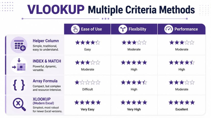
A practical comparison

Method	Best fit	Main advantage	Main drawback
Helper Column + VLOOKUP	Older Excel, simple models	Easy to teach and audit at first glance	Adds extra columns and duplicated keys
INDEX + MATCH	Users comfortable with formulas	Flexible without changing source data	Harder to read and debug
XLOOKUP	Modern Excel, single return value	Cleaner formula logic	Not available in older environments
FILTER	Modern Excel, multiple matching rows	Returns full result sets automatically	Spill range can collide with other cells

Performance is not a small detail

The helper-column method is often taught as the default workaround, but on large datasets it can become a bottleneck. Guidance on this point is blunt: duplicated data in helper columns increases file size, slows recalculation cycles, and requires manual maintenance (DataCamp discussion of helper-column performance issues).

That matters most when:

• Files update often: New rows require the helper formula to stay consistent.
• Several tabs depend on the same keys: You multiply maintenance work.
• The workbook is already heavy: Extra calculated text columns don't help.

If your file is slowing down, it's worth pairing formula cleanup with workbook cleanup. This guide on how to compress Excel files is useful when helper columns and repeated formulas have inflated the file more than expected.

Maintainability usually decides the winner

A formula that works today can still be the wrong choice if no one wants to touch it later.

Complex nested lookup logic creates a real documentation problem in shared workbooks. Someone inherits the file, sees a long array formula, and becomes afraid to edit anything. That's where technical debt starts showing up in Excel.

Here's the decision framework I use most often:

• Choose helper columns when the workbook is small, the team uses mixed Excel versions, and clarity matters more than elegance.
• Choose INDEX/MATCH when you must keep source data unchanged and the person maintaining the workbook understands array logic.
• Choose XLOOKUP when your team has modern Excel and each search should return one clear answer.
• Choose FILTER when you need all matches, not just the first one.

The best formula isn't the shortest one. It's the one the next analyst can still trust.

A realistic workflow check

A lot of teams don't work only in Excel. They move data between Sheets, marketplaces, exports, and reporting files. If your lookup logic depends on imported e-commerce data, a practical reference on Amazon data in Google Sheets can help you think through where the data should be cleaned before it even reaches Excel.

That's an underrated point. Sometimes the smartest multi-criteria lookup fix is upstream data cleanup, not a more complicated formula.

The 1-Minute Solution Automate Lookups with AI

The hardest part of multi-criteria lookup work usually isn't writing one formula once. It's maintaining that logic when the workbook changes, the criteria expand, or another person inherits the file.

Microsoft has highlighted the maintenance burden around multi-criteria lookup formulas, especially when nested logic becomes difficult to audit, modify, or explain in shared workbooks (Microsoft discussion of multiple-criteria lookup formula complexity).

That's where AI starts to matter inside Excel. Instead of remembering whether this workbook needs helper columns, INDEX/MATCH, or FILTER, you can describe the result you want in plain language and let the tool handle the mechanics.

For example, an Excel AI agent can take a request like “find the matching price for this product and region, then fill the result down the column” and execute the lookup workflow directly. That's different from a formula explainer. It shifts the work from formula construction to task execution.

This is also the same reason automation matters outside spreadsheets. If your process includes pulling values from invoices, forms, or PDFs before the data even reaches Excel, tools for document processing automation can remove a separate layer of manual lookup work.

If you want that same automation approach inside spreadsheets, Excel AI as a VBA alternative is the right frame to think in. Elyx AI is one example. It works as an Excel add-in that executes spreadsheet tasks from natural-language requests, so the lookup becomes part of a larger workflow instead of one more formula someone has to maintain.

---

If you're tired of patching together helper columns, array formulas, and spill ranges, Elyx AI gives you another option inside Excel. You describe the lookup or reporting task in plain English, and the agent executes the workflow directly in the sheet. That's useful when the actual problem isn't just finding the right formula. It's keeping the workbook usable after the formula is in place.