How to Connect Sheets in Excel: A Practical Guide

If you've ever spent hours manually copying and pasting data from one Excel sheet to another, you know how mind-numbing and error-prone it can be. Mastering how to connect sheets in excel isn't just a neat trick; it's a fundamental skill that transforms your spreadsheets from static documents into a dynamic, interconnected system. This approach saves a massive amount of time and, more importantly, prevents the kind of costly mistakes that creep in with manual data entry.

Why Connecting Excel Sheets Is a Business Superpower

Think about how data flows in a typical company. The finance team has its sales reports, project managers track individual contributions in separate tabs, and marketing has its own performance metrics. When this information lives in isolated silos, you’re constantly chasing down the latest numbers and hoping nobody made a typo along the way.

Linking your spreadsheets correctly solves this problem by creating a 'single source of truth'. This is a simple but powerful concept: when the original data is updated, every report, chart, and summary that relies on it updates automatically. It’s the key to maintaining data integrity and trusting the numbers you’re looking at.

The True Cost of Disconnected Data

Spreadsheets are the lifeblood of the modern workplace. It’s not uncommon for office workers to have an average of 2.6 spreadsheets open at any given time. What's truly staggering is that they spend about 38% of their day just working within these files. This is according to an insightful in-depth Microsoft 365 report on workplace habits.

When those spreadsheets aren't connected, that time sink gets much worse. Every time a sales figure changes, someone has to manually find every place it's referenced and update it. This isn't just slow—it's practically an invitation for errors. A single copy-paste mistake can throw off an entire forecast, leading to poor business decisions.

The real goal is to spend less time wrangling data and more time analyzing it. When you connect your sheets, you automate the grunt work. This frees you up to focus on what actually matters: finding insights and making smart decisions with accurate, current information.

This principle is a cornerstone of What Is Business Intelligence and is essential for effective data management. If you're looking at the bigger picture, our business intelligence software comparison explores how this concept of connected data scales up to power more advanced analytical tools.

Linking Data Inside a Single Workbook

The foundation of connecting data in Excel lies in mastering the basics within a single workbook. These techniques are essential for creating smarter, automated reports and are quick to learn.

The most straightforward way to pull data from one sheet to another is with a direct cell reference. Let's say you have a "Summary" sheet and need to display the final sales total, which is located in cell F50 on your "SalesData" sheet.

On your "Summary" sheet, click a cell and type:
=SalesData!F50

This formula tells Excel to go to the sheet named 'SalesData' and return the value from cell F50. The exclamation mark ! separates the sheet name from the cell address. This creates a live link, perfect for dashboards where you need to pull specific KPIs from different tabs.

Consolidating Data with 3D References

What if you have multiple sheets with the exact same layout? Imagine a workbook with a separate sheet for each month—Jan, Feb, and Mar. If you want to sum the total expenses from cell B10 across all three months, you don't need a cumbersome formula like =Jan!B10 + Feb!B10 + Mar!B10.

This is where 3D references are incredibly useful. Instead, you can use one clean formula:
=SUM(Jan:Mar!B10)

This formula sums the value in cell B10 across all sheets from 'Jan' to 'Mar', inclusive. The colon : between the sheet names creates the 3D range. The only requirement is that the sheets must be positioned consecutively in the workbook. It's an efficient way to create quarterly or annual roll-up summaries from monthly data.

Pro Tip: If you drag a new, identically formatted sheet (e.g., 'Feb_Bonus') and drop it between the 'Jan' and 'Mar' tabs, Excel automatically includes it in the SUM. Your report updates itself, which is a huge time-saver.

Making Formulas Readable with Named Ranges

As your spreadsheets grow, formulas like =SUM(SalesData!F2:F50) can become confusing. It's tough to remember what F2:F50 represents. This is precisely the problem Named Ranges solve. A Named Range allows you to assign a descriptive name to a cell or a range of cells, making your formulas instantly understandable.

To create one, highlight the cells you want to name (e.g., all your Q1 sales figures on the "SalesData" sheet). Then, go to the Name Box—the small box to the left of the formula bar—type a name like Q1_Sales, and press Enter.

Now, your formula transforms from something cryptic into this:
=SUM(Q1_Sales)

This simple practice makes your workbooks dramatically easier for you and your colleagues to read, debug, and maintain.

---

Choosing the Right Internal Linking Method

Deciding which method to use can be tricky. Here’s a quick comparison to help you choose the right tool for the job.

Method	Best For	Example Syntax	Key Advantage
Direct Cell Reference	Pulling a single, specific value from another sheet. Ideal for dashboards and summaries.	=Sheet2!A1	Simple, fast, and creates a direct link to a single piece of data.
3D Reference	Aggregating data (SUM, AVERAGE, etc.) from the same cell across multiple, identically structured sheets.	=SUM(Jan:Mar!B10)	Consolidates data from many sheets with one concise formula.
Named Range	Making complex formulas easy to read and manage, especially in large models.	=SUM(Q1_Sales)	Improves formula clarity and makes the workbook much easier to maintain.

Each method has its place. Direct references are for simple one-off links, 3D references are for roll-ups, and Named Ranges bring clarity and professionalism to your models. For more dynamic data retrieval based on specific criteria, you'll want to explore lookup functions. Our detailed guide on how to use INDEX MATCH is a great next step.

Using Lookup Formulas to Pull Data Dynamically

When a simple, static link isn't enough, lookup formulas are the solution. They allow you to connect sheets in Excel intelligently. Instead of grabbing data from a fixed cell, these formulas search for a specific piece of information in one table and pull in related data from another. This is the logic behind interactive dashboards and automated data entry.

For example, imagine you have a master HR sheet with employee details and a separate departmental budget sheet. Your goal is to pull each employee's salary from the master list into the budget sheet, matching them by their unique employee ID. This is a classic problem that lookup formulas solve perfectly.

The Classic Approach: VLOOKUP

For years, VLOOKUP (Vertical Lookup) was the standard for this task. It searches for a value in the first column of a table and returns a corresponding value from another column in the same row. While it has limitations, understanding VLOOKUP is essential for any Excel user.

Let's use our HR example. Your 'Budget' sheet has employee IDs in column A. The 'HR_Master' sheet has all employee data, with IDs in column A and their salaries in column D.

To pull the salary into the 'Budget' sheet, you would use this formula in cell B2:
=VLOOKUP(A2, HR_Master!A:D, 4, FALSE)

Here is a detailed breakdown of the formula:

• A2: This is the lookup_value—the unique employee ID you're searching for.
• HR_Master!A:D: This is the table_array where Excel will search. The lookup value must be in the first column of this range (column A).
• 4: This is the col_index_num. Since 'Salary' is the 4th column in the A:D range, Excel will return a value from this column.
• FALSE: This specifies the range_lookup type, demanding an exact match. You should almost always use FALSE to prevent incorrect matches.

The Flexible Alternative: INDEX and MATCH

VLOOKUP’s main weakness is that it can only look to the right. If the salary data were in a column to the left of the employee IDs, VLOOKUP would fail. That’s where the powerful combination of INDEX and MATCH comes in.

This two-part formula is far more flexible. MATCH finds the position (the row number) of a value in a column, and INDEX then retrieves the value from that same position in a different column.

Using the same scenario, the formula would be:
=INDEX(HR_Master!D:D, MATCH(A2, HR_Master!A:A, 0))

Here’s how they work together:

• MATCH(A2, HR_Master!A:A, 0): This part finds the employee ID from cell A2 within the ID column (A:A) on the master sheet. The 0 ensures an exact match. If it finds the ID in row 55, it returns the number 55.
• INDEX(HR_Master!D:D, ...): INDEX then takes that position number (55) and goes to the 55th cell in the salary column (D:D) to retrieve the correct value.

This combination is a favorite of Excel professionals because it is not dependent on column order and doesn't break if you insert or delete columns.

The Modern Powerhouse: XLOOKUP

Microsoft introduced a modern successor that combines the best of both worlds: XLOOKUP. It has the simplicity of VLOOKUP and the flexibility of INDEX/MATCH. For anyone with a recent version of Excel, this is the recommended function.

The XLOOKUP formula for our example is refreshingly simple:
=XLOOKUP(A2, HR_Master!A:A, HR_Master!D:D)

Let's break it down:

• A2: The lookup_value you're searching for.
• HR_Master!A:A: The lookup_array, the column to search in.
• HR_Master!D:D: The return_array, the column to pull the result from.

XLOOKUP is cleaner to write, more efficient, and defaults to an exact match, which prevents many common VLOOKUP errors. It also has built-in error handling, allowing you to specify what to return if a value isn't found, all within one function.

To fully master this function, check out our complete guide on how to use XLOOKUP in Excel, which covers everything from the basics to more advanced applications.

Connecting Data Across Different Excel Workbooks

When your data is split across separate files, you need to create an external link. This is crucial for building consolidated dashboards that pull information from multiple sources, such as a master sales report that aggregates data from individual regional files.

The process is straightforward. Start a formula with = in your main workbook, then switch to the source workbook, click on the desired sheet and cell, and press Enter.

Excel automatically generates the syntax, which includes the full file path:
='[RegionalSales.xlsx]Q1'!$B$5

This formula tells Excel to get the value from cell B5 on the sheet named 'Q1' inside the workbook named 'RegionalSales.xlsx'. The link's integrity depends entirely on the name and location of that source file.

Managing and Repairing External Links

This dependency is a common source of problems. If you rename or move the source workbook, your link will break, and you'll see the #REF! error.

Fortunately, Excel provides a central hub for managing these connections:

• Go to the Data tab on the ribbon.
• In the Queries & Connections group, click Edit Links.
• A window will appear, listing every external file your workbook is linked to.
• Select the broken link (it will usually have an error status) and click Change Source.
• Browse to the file’s new location to repair the connection.

Think of the 'Edit Links' window as your command center for all external data. Regularly checking it can help you catch problems early and maintain the integrity of your reports.

Best Practices for Robust Workbook Connections

A little planning can save you from the future hassle of fixing broken links. The best practice is to create a logical and consistent folder structure, especially on a shared network drive. Keep all related workbooks inside a single parent folder before you start linking them. This way, if you need to move the entire project, all relative file paths move with it and remain intact.

For more complex setups, automating these data pipelines can dramatically reduce manual errors. If this sounds interesting, you might want to explore the broader topic of the automation of Excel tasks, which offers powerful ways to manage these data flows.

Automating Connections With Power Query

When you need a robust way to connect sheets in Excel that goes beyond simple cell links, it's time to learn Power Query. Built into modern Excel versions (on the Data tab, in the "Get & Transform Data" group), it is the best tool for consolidating and cleaning data from multiple sources without writing complex formulas.

Imagine you have separate Excel files for each month's sales data. Manually copying and pasting that information together is tedious and prone to errors. With Power Query, you can simply point it to a folder containing all 12 files. It will automatically combine them into one clean, consolidated master table.

This diagram illustrates the basic concept of linking workbooks by pulling data from a source file into a master file.

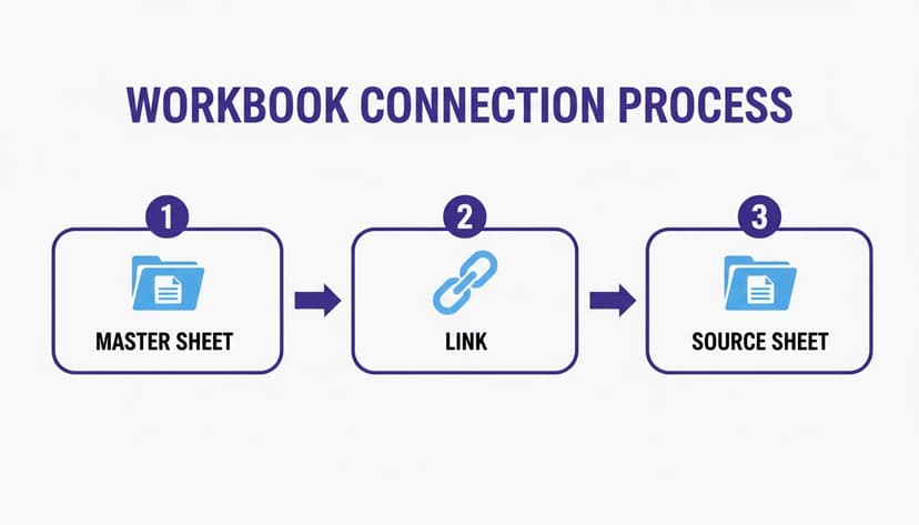
Power Query enhances this concept, allowing you to connect to entire folders of files, not just individual cells.

The Refreshable Magic of Power Query

The true power of Power Query lies in its "set it and forget it" nature. Once you build a query to combine your monthly sales files, that process is saved as a series of steps. Next month, when you add the March report to the folder, you just open your master workbook and click "Refresh All." Power Query automatically reruns all the steps, pulling in the new data seamlessly.

This approach transforms your Excel file from a static report into a dynamic, self-updating dashboard. You build the data pipeline once, and it handles the rest, saving countless hours and eliminating human error.

Tools like Power Query have revolutionized data handling in Excel. Yet, with 345 million paid Microsoft 365 subscribers and office workers spending 38% of their time in spreadsheets, inefficient processes represent a significant hidden cost.

Beyond Simple Merging: Data Transformations

Power Query is more than just a tool for combining files; it’s a full-fledged data transformation engine. The Power Query Editor provides a user-friendly interface to perform hundreds of operations to clean and shape your data before it even reaches your worksheet.

Here are a few examples of what you can do:

• Remove columns you don't need to keep your final table clean.
• Filter rows that don't meet certain criteria (e.g., removing returns from a sales report).
• Split a single column into several (e.g., "Full Name" into "First Name" and "Last Name").
• Add custom columns based on your own calculations (e.g., a "Commission" column based on sales figures).

This ability to clean data at the source ensures your final report is always accurate and ready for analysis. To learn more, check out our guide on how to automate Excel reports. You can also pair Power Query with other tools like Power Automate for Non-Technical Teams to connect your Excel workflows to other business processes.

Got Questions? We've Got Answers

Connecting sheets in Excel is powerful, but it can raise a few common questions. Let's tackle them so you can move forward with your analysis.

What’s the Best Way to Connect More Than Ten Sheets?

When you need to consolidate data from a large number of identically structured sheets (more than ten), the best solution is Power Query.

While 3D references are fine for a quick SUM across a few tabs, they become slow and difficult to manage as the number of sheets increases. Power Query, on the other hand, is designed for this task.

With Power Query, you can:

• Connect to an entire folder and import every Excel file within it.
• Consolidate all sheets from your current workbook.
• Append all the data into a single, clean master table.

The best part is its refreshable nature. When you add new sheets, a simple click on "Refresh" updates your entire dataset. It is a far more scalable and robust solution than managing complex formulas.

How Do I Fix Broken Links When I Move an Excel File?

Broken links are a common issue when you move or rename a source workbook that is linked to another file. Fortunately, the fix is simple.

Navigate to the Data tab and click the Edit Links button in the "Queries & Connections" group.

A dialog box will appear, listing all your external source files. Find the broken link (Excel will usually flag it with an error), select it, and click Change Source. Then, simply browse to the file's new location to restore the connection.

Pro Tip: To prevent this issue, always store related workbooks in the same folder before you create links between them.

Can I Connect an Excel Sheet to a Google Sheet?

Yes, you can, although it requires a workaround. The most reliable method is to publish your Google Sheet to the web as a CSV file.

Here's the process:

1. In your Google Sheet, go to File > Share > Publish to web.
2. Choose the specific sheet you want to share and select "Comma-separated values (.csv)" as the format.
3. Click "Publish" and copy the generated URL.

Next, return to Excel. Go to the Data tab, click From Web, and paste the URL. Power Query will open, allowing you to import and transform the data. This creates a refreshable, read-only connection to your Google Sheet.

---

Still spending too much time on manual Excel work? With Elyx AI, you can describe what you need in plain English—like "Consolidate these sales sheets, create a pivot table by region, and format the report"—and our AI agent gets it done for you right in your spreadsheet. Stop fighting with formulas and start getting answers faster.

Try Elyx AI for free and automate your Excel tasks today