Master the Annuity Formula Excel: Step-by-Step Guide 2026

You're probably in one of two situations right now. Either you need a clean monthly payment for a loan model, or you're trying to value a stream of recurring cash flows without building a messy spreadsheet from scratch.

That's where annuity formula excel work stops being academic and becomes practical. Loans, leases, retirement savings, pension projections, sinking funds, and payment plans all rely on the same core idea: cash flows repeat over time, and timing matters. If you get the rate, period count, or payment timing wrong, the model looks polished but gives the wrong answer.

Excel is still the fastest place to solve this. Its built-in financial functions handle the math directly, and they're far safer than hand-built formulas spread across ten tabs. The primary challenge isn't finding a formula. It's knowing which function to use, how to set the inputs correctly, and where the common traps are hiding.

Why Mastering Annuity Formulas in Excel is a Superpower

A quarterly close goes sideways faster than people expect. A model uses an annual discount rate against monthly cash flows, lease payments are set to end-of-period when the contract says beginning-of-period, and the sign on PMT flips halfway through a schedule. The workbook still looks clean. The answer is still wrong.

That is what makes annuity formulas so useful in Excel. They turn recurring cash flow math into a controlled process instead of a chain of hand-built calculations scattered across a model. For this reason, Excel's time-value-of-money functions became a fixture in day-to-day finance work once they were built into standard spreadsheet workflows. The benefit is not academic elegance. It is fewer avoidable errors in pricing, valuation, debt schedules, and savings forecasts.

The primary advantage is speed with discipline. A good analyst can test a refinance case, resize a lease payment, or compare contribution scenarios in minutes without rebuilding the logic each time. That matters in live work, where the delay usually comes from checking assumptions and cleaning spreadsheet mechanics, not from the finance theory itself.

Practical rule: If cash flows repeat and the rate is stable, start with Excel's financial functions before building custom formulas.

The stronger payoff shows up in the messy cases that basic tutorials skip. Growing contributions, deferred start dates, and mismatched compounding versus payment frequencies are common in actual models. They also create the kinds of quiet errors that survive review because the formula looks plausible. Analysts who know how Excel handles those cases save time and catch problems earlier.

There is also a workflow trade-off. Building annuity logic manually gives full control, but it is slow to audit and easy to break when assumptions change. Using Excel's built-in functions cuts that risk, and pairing them with automation cuts it further. A practical example is this guide to Excel AI for financial modelling, which shows how ElyxAI can generate formula structures, check period alignment, and reduce the repetitive setup work so you can spend more time on assumptions, review, and decisions.

The 5 Core Excel Annuity Functions Explained

A lot of annuity work in Excel comes down to one practical question: which variable is missing? If the missing piece is the payment, use PMT. If it is today's value, use PV. If it is the ending balance, use FV. If you need the implied return, use RATE. If the open question is time, use NPER.

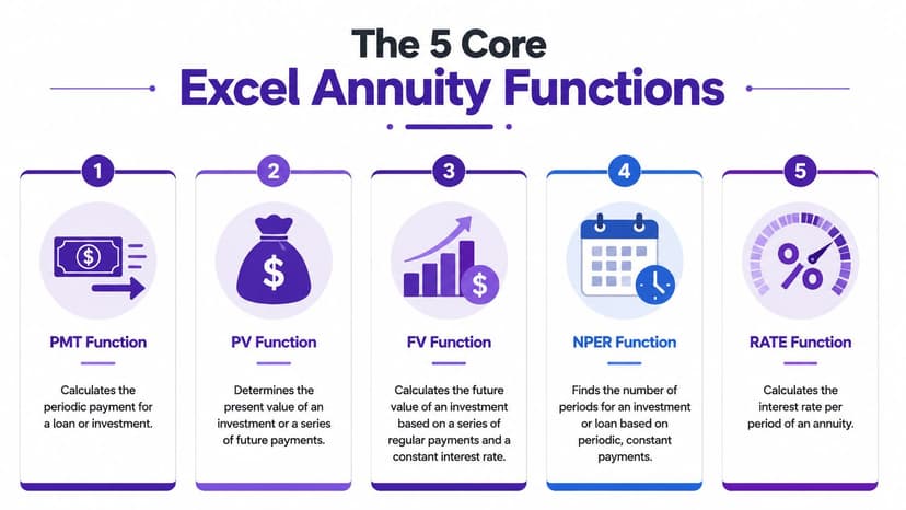
That sounds basic. In practice, getting this mapping right saves a lot of rework, especially in models that later expand into growing annuities, deferred cash flows, or frequency mismatches.

Quick reference table

Function	What it solves	Basic syntax	Typical use
PMT	Periodic payment	=PMT(rate,nper,pv,[fv],[type])	Loan instalments, savings contributions
PV	Present value today	=PV(rate,nper,pmt,[fv],[type])	Valuing an annuity, lease, pension stream
FV	Future value later	=FV(rate,nper,pmt,[pv],[type])	Savings plans, retirement models
RATE	Interest rate per period	=RATE(nper,pmt,pv,[fv],[type])	Solving for implied return or borrowing cost
NPER	Number of periods	=NPER(rate,pmt,pv,[fv],[type])	Time needed to repay debt or hit a target

Excel has had these functions for decades, and there is a reason analysts still rely on them. They are fast, consistent, and easier to audit than custom annuity formulas scattered across a workbook.

PMT for payment amounts

Use PMT when the cash flow amount is unknown and everything else is set.

That is the standard setup for mortgages, car loans, leases, and recurring savings plans. If you know the rate per period, the number of periods, and the starting balance, PMT returns the fixed payment required. Excel will usually show a negative result for a loan payment because it treats that payment as a cash outflow. That is not an error. It is sign convention doing its job.

A simple mortgage quote, for example, often starts with the same logic used in a simulateur de prêt immobilier expatrié. The difference is that Excel lets you expose every assumption and test alternatives instead of accepting a single black-box result.

PV for valuing future payments

Use PV when the payment stream is known and you need its value today.

That shows up in pension analysis, lease valuation, structured settlement reviews, and any case where equal payments arrive over time. A compact example is =PV(8%/12,120,100). Excel discounts 120 monthly payments of 100 at a monthly rate derived from 8% per year and returns the present value of that annuity.

The main mistake here is period mismatch. If the payments are monthly, the rate must be monthly and the term must be stated in months. If one input stays annual while the others are monthly, the output can look reasonable and still be wrong.

FV for savings and accumulation

Use FV when you need to project where recurring deposits will end up.

For example, =FV(6%/12,120,-500) estimates the ending value of contributing 500 per month for 10 years at 6% annually, compounded monthly. This method cleanly separates three levers: contribution amount, rate, and time. That makes it useful for savings models because you can stress-test behavior changes without rewriting the structure.

It is also where basic guides usually stop. Real planning models often need step-ups in contributions, skipped periods, or different compounding and contribution frequencies. Excel can handle that, but the setup moves beyond a single FV formula.

A practical shortcut: PMT solves for the cash flow, PV for today's value, FV for the ending value, RATE for the return, and NPER for the timeline.

RATE for implied returns

RATE works backward. You know the cash flows and target value, but not the return that connects them.

That makes it useful for checking quoted products, evaluating savings targets, and testing whether a proposed repayment plan is internally consistent. A formula like =RATE(10,-7500,0,100000) solves for the periodic rate implied by ten equal contributions and a final target value.

RATE deserves more caution than the other four functions. It is an iterative calculation, so unusual inputs or poor sign handling can produce errors or a result that converges to the wrong place. In review work, I usually sanity-check RATE against a rough estimate before I trust it.

NPER for time horizons

NPER answers the question decision-makers ask constantly and spreadsheets often bury: how long will this take?

Use it for payoff timing, savings milestones, and retirement income planning. If rate, payment, and balance are fixed, NPER returns the number of periods required to reach the target. That is useful when a plan looks affordable on a monthly basis but unrealistic once timing is made explicit.

If you are building these formulas from scratch, a clear refresher on how to make a formula in Excel helps before you combine financial functions with IF logic, named ranges, and scenario inputs. ElyxAI also helps on the repetitive side of this work by generating formula drafts, checking sign consistency, and flagging period mismatches before they spread through the model.

How to Calculate Payments and Build a Loan Schedule

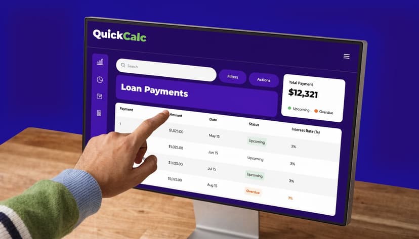
For loan work, PMT is the anchor formula. Once you trust the payment calculation, you can split that payment into interest and principal and build an amortization schedule that explains what's happening over time.

Start with the payment formula

A standard structure looks like this:

• Rate per period: annual rate divided by payment frequency
• Number of periods: years multiplied by payment frequency
• Present value: original loan balance
• Future value: usually 0 for a fully repaid loan
• Type: 0 for end-of-period payments unless the contract says otherwise

A practical PMT formula is:

=PMT(rate, nper, pv, 0, 0)

If you're working with a monthly mortgage, the logic is straightforward. Convert the annual rate to a monthly rate and convert the loan term to monthly periods. The result is the fixed monthly payment.

One of the biggest failure points is sign handling. According to Exceljet's payment for annuity reference, sign convention errors account for up to 60% of incorrect results in user-created models, and using Excel's built-in functions correctly can cut modeling errors by 92% compared with manual calculations.

Modeling habit: Decide upfront which values are inflows and outflows, then keep that convention consistent across PMT, IPMT, PPMT, PV, and FV.

If you're checking assumptions against an external calculator before finalizing a workbook, a targeted tool like this simulateur de prêt immobilier expatrié can be helpful for cross-checking repayment logic in real estate contexts.

Build the amortization schedule

Once PMT is working, create a schedule with at least these columns:

Column	Purpose
Period	Payment number
Opening balance	Loan balance at start of period
Payment	Fixed total payment from PMT
Interest	Interest portion for that period
Principal	Principal repaid in that period
Closing balance	Remaining balance

The interest and principal split typically uses IPMT and PPMT. The payment stays constant, but the composition changes over time. Early periods are more interest-heavy. Later periods repay more principal.

That's where a schedule becomes useful, not just decorative. It shows when the balance starts moving meaningfully and makes it easier to test refinance scenarios, prepayments, and sensitivity to term changes.

A walkthrough can help if you want to see the mechanics in action:

What works in real models

The best loan sheets are usually the simplest ones. They keep assumptions in one input block, avoid hard-coded values inside formulas, and reference named cells or clearly labeled assumptions.

Three habits save a lot of rework:

1. Keep units aligned. Monthly rate with monthly periods. Annual rate with annual periods.
2. Separate inputs from calculations. Don't bury assumptions inside the schedule.
3. Check the ending balance. A properly built amortization table should bring the closing balance to zero, or very close due to rounding.

If you want a prebuilt structure instead of constructing the table manually, this loan amortization calculator gives you a clean reference point for layout and logic.

How to Project Your Savings and Future Wealth

A savings model usually starts with a simple question from a client, a manager, or your own planning sheet. If I contribute a fixed amount every month, what does that turn into by retirement, a home purchase date, or the end of a 10-year plan? In Excel, FV is the function that answers it fast.

Use FV to model recurring contributions

The basic form is:

=FV(rate, nper, pmt, [pv], [type])

For a standard contribution plan, set pv to zero if you are starting from scratch, enter contributions as a negative number, and keep the rate and period count on the same frequency. A clean example is:

=FV(6%/12, 120, -500, 0, 0)

That formula projects the future value of monthly contributions over 10 years at a 6% annual return assumption, with deposits made at the end of each month.

The sign convention matters more than many guides admit. If you enter the contribution as positive, Excel will often return a negative future value. The math is still internally consistent, but the output is harder to read and easy to misinterpret in client-facing models.

Focus on the inputs that actually move the result

Three assumptions do most of the work in accumulation models:

• Contribution amount
• Time invested
• Rate of return

Time usually has the biggest effect because each early deposit gets more periods to compound. That is why a modest contribution increase made early can matter more than a late attempt to catch up with larger deposits.

A one-cell FV formula is fine for a quick answer. A decision-ready model usually needs more. Build the sheet so you can test a base case, a conservative case, and an upside case without rewriting formulas.

Build for planning, not false precision

Good savings projections are flexible enough to handle realistic planning questions. What happens if contributions rise every year with salary? What if deposits are made at the start of the month? What if accumulation runs monthly but the return assumption is set annually? Those are the actual workbook problems, and they are exactly where basic tutorials stop too early.

For retirement work, context matters as much as the formula. If your model supports pension drawdown or retirement income planning, this overview of Everglow Prosperity financial advice adds useful background on account-based pension decisions alongside the Excel math.

If you also need to compare contribution-based growth with annualized performance, this guide to the CAGR formula in Excel is a useful companion.

I usually recommend one extra layer in the workbook. Add a small sensitivity table that changes return assumptions by 1% to 2% and contribution levels by a fixed monthly amount. That exposes whether the plan is being driven by disciplined saving or by an aggressive return assumption.

ElyxAI helps when the model stops being a single FV formula and turns into a messy planning sheet. It can generate scenario tables, catch mismatched frequencies, and flag sign errors before they roll into a retirement projection that looks precise but is built on the wrong setup.

3 Advanced Annuity Scenarios Most Guides Ignore

Real-world annuity models break in predictable places. Timing shifts by one period, payments grow over time, or the cash flow schedule does not match the compounding schedule. Basic Excel examples rarely cover those cases well, yet they show up constantly in lending, retirement planning, lease work, and treasury models.

1. Ordinary annuity versus annuity due

This is the first distinction that changes the answer without changing much of the formula. An ordinary annuity assumes cash flows occur at the end of each period. An annuity due assumes they occur at the beginning.

In Excel, the switch usually sits in the type argument:

• 0 = end of period
• 1 = beginning of period

That input looks minor. It is not. Earlier cash flows carry more value, so the present value of an annuity due will be higher than the same payment stream modeled as an ordinary annuity.

A quick check makes the point. Compare:

=PV(8%/12,120,100)

with:

=PV(8%/12,120,100,0,1)

The formulas differ only by type=1, but the result changes because every payment is pulled forward by one period. I see this error often in rent schedules, equipment leases, and contribution models where the first deposit happens immediately. If the agreement says payment is due upfront, leaving Excel at the default 0 can understate value.

2. Growing annuities

Level-payment examples are useful for learning, but a lot of live models are not level. Pension income may include annual increases. Service contracts may escalate by a fixed percentage. Savings plans often rise with salary.

Excel does not have a dedicated built-in growing annuity function, so the formula has to be written directly:

=C1/(r-g)*(1-((1+g)/(1+r))^n)

Here:

• C1 is the first payment
• r is the discount rate
• g is the growth rate
• n is the number of periods

A practical check helps avoid bad outputs. Keep the units aligned first. If r is annual, g and n need to be annual too, unless you intentionally convert the whole setup to monthly or quarterly terms. The second check is conceptual. If g ≥ r, the valuation becomes unstable or economically unrealistic for many planning cases, and Excel may return an error or a misleading result.

This is also where analysts waste time rebuilding the same sensitivity grid by hand. If the model needs several growth assumptions, discount rates, and term lengths, structured what-if analysis in Excel is the better way to test the range instead of editing cells one by one.

3. Mismatched payment and compounding frequencies

A lot of annuity mistakes come from mixing schedules. The contract may pay quarterly while interest compounds monthly. A return assumption may be quoted annually, but the workbook calculates monthly deposits. Those are not edge cases. They are standard finance work.

Typical examples include:

• quarterly payments with monthly compounding
• annual withdrawals with semiannual compounding
• monthly contributions paired with a nominal annual rate

The common shortcut is to divide the annual rate by the number of payments and use that everywhere. Sometimes that is acceptable. Often it is not. Payment frequency and compounding frequency are separate assumptions, and collapsing them into one rate can distort both valuation and projected balances.

A better approach is to convert the stated annual rate into the effective rate that matches the cash flow timing, then run the annuity formula on that basis. In Excel, that usually means using EFFECT, NOMINAL, or an explicit periodic-rate conversion before applying PV, FV, or PMT. The extra step matters most in longer-dated models, where small periodic differences accumulate into a material gap.

Handling these repetitive setups is a task where an AI assistant inside Excel can save meaningful time. ElyxAI can map the timing structure, generate the converted-rate formulas, and build scenario tabs from a plain-language prompt. That does not replace judgment on assumptions. It cuts down the manual setup errors that tend to survive until review.

6 Common Annuity Formula Pitfalls and How to Fix Them

Bad annuity models usually do not fail loudly. They produce a number that looks plausible, gets pasted into a deck, and only surfaces later when a payment quote, reserve estimate, or savings projection does not reconcile.

I see the same errors repeatedly in loan models, retirement projections, and lease workbooks. The fix is rarely complicated. The hard part is knowing where Excel is doing exactly what you asked instead of what you meant.

1. Sign convention confusion

Symptom: PMT, PV, or FV returns a negative number when you expected a positive one.

Cause: Excel assumes one side of the cash flow is an outflow and the other is an inflow. The function is not wrong. The model perspective is unclear.

Fix: Set the perspective before writing formulas. If the model is from the borrower's view, payments are outflows and should usually be negative. If the model is from the lender's view, those same payments are inflows. Do not fix one cell by wrapping it in a minus sign unless you apply that logic consistently across the schedule.

2. Rate and period mismatch

Symptom: Payment amounts or future values look obviously too high or too low.

Cause: The rate and number of periods are expressed in different units. A common example is using an annual rate with monthly periods, or using 60 periods for a 5-year loan while leaving the rate annual.

Fix: Match both inputs to the same time base every time. Monthly cash flows require a monthly rate and a monthly period count. This is the first thing to audit because a clean-looking workbook can still be off by a wide margin if the time units are mixed.

3. Wrong type argument

Symptom: The answer is close, but consistently off for rent, lease, or deposit models.

Cause: Excel defaults type to 0, which means end-of-period payments. Many real cash flows happen at the beginning of the period.

Fix: Use type=1 for annuities due. That one argument changes valuation, payment sizing, and schedule timing. In practice, I check this anywhere cash leaves or arrives on day one of the period rather than at period end.

Timing errors are small in one period and material across many periods.

4. Using standard annuity logic for growing payments

Symptom: Pension income, tuition plans, inflation-linked withdrawals, or stepped lease payments are misvalued.

Cause: Standard Excel annuity functions assume level payments. They do not directly handle cash flows that grow each period.

Fix: Build the growth explicitly. In some cases that means using a growing annuity formula outside the core Excel functions. In other cases, it means projecting each payment row by row and discounting the stream directly. The second method is slower to build but easier to audit, which matters when growth assumptions are contentious or variable.

5. Mishandling mismatched frequencies

Symptom: The model appears internally consistent, but results still do not tie to the contract or expected economics.

Cause: Payment timing and rate application are being forced into the same frequency even when they are different. This often happens in products with quarterly payouts, monthly accrual, or annual contribution assumptions converted too casually.

Fix: Convert the rate to the cash flow frequency before using PMT, PV, or FV. As noted earlier, EFFECT, NOMINAL, or an explicit periodic-rate conversion earns its keep in these situations. The shortcut of dividing the annual rate by the payment count is fast, but it is not always accurate enough for long-dated models or pricing work.

6. Ignoring Excel error messages

Symptom: #NUM! or #VALUE! shows up and the model stalls.

Cause: The workbook has an input problem, not a formatting problem. Typical causes include text stored as numbers, missing arguments, inconsistent signs, or assumptions that break the math. Growing annuity setups are especially sensitive if growth is at or above the discount rate.

Fix: Audit inputs before touching formula syntax. Check data types, signs, timing, and assumption order. If the model still fails, test the formula on a simple known case first, then add complexity back one input at a time.

A short review routine catches most of these problems before they make it into a final model:

• Check units first. Rate frequency, payment frequency, and term must align.
• Confirm the type input for every payment stream.
• Trace signs across the full model instead of fixing a single output cell.
• Test one simple case manually to confirm the workbook logic.
• Separate assumptions from formulas so review is faster and changes are safer.

Elyx AI helps with the repetitive part of this work inside Excel. It can generate formulas, build schedules, and structure scenario tabs from plain-language instructions. That saves time, but its true value is reducing setup mistakes before they get buried in a larger workbook.