How to Sort Data in Excel Efficiently and Quickly

Quick Answer For Sorting Data In Excel

Excel hands you everything from a simple A–Z click to a formula-driven list. You can reorganize data instantly or build a live sort that updates on the fly—often accelerated by AI assistants like Elyx.AI or Excel’s own Copilot.

• Click the A–Z or Z–A buttons to reorder a single column in seconds
• Hit the Sort dialog with Alt+D+S to stack multiple levels
• Turn your range into a table so new rows follow the same sort rules
• Use the SORT() function for dynamic, auto-updating lists
• Sort by cell color, font color, or icon sets to spot trends

Key Takeaway: Match your sorting approach to your data shape and objectives for instant clarity.

Spending too much time on Excel?

Elyx AI generates your formulas and automates your tasks in seconds.

Try for free →

Sorting Methods Summary

Below is a quick rundown of common Excel sorting techniques and when to use each one.

Method	Use Case	Keyboard Shortcut
Single-Column Sort	Alphabetize or rank one column	Alt+A+S+S
Multi-Level Sort	Preserve relationships across columns	Alt+D+S
Dynamic SORT Formula	Keep lists updated automatically	—
Color Or Icon Sort	Highlight status or priority visually	—

Pick the method that matches your dataset and goal for instant results. Dive deeper into advanced sort tricks and dynamic SORT formulas and AI workflows on our detailed guide.

Understanding Basic Sorting Techniques

Excel makes it easy to rearrange your data whether you’re working in a simple range or a fully formatted table. You can tap the A–Z or Z–A buttons on the ribbon and see instant results.

Imagine you have a customer list—first by purchase date, then by region—and want to spot trends. Tables will automatically apply those sort rules whenever you add new entries, saving you from repetitive clicks.

Common sorting moves include:

• Clicking A–Z or Z–A on the Home tab for one-click sorts
• Pressing Alt+D+S to launch the Sort dialog in a flash
• Adding levels in that dialog to lock in multiple criteria
• Converting a range into a table so new rows follow your sort order

Ever since Excel first let us reorder columns back in 1985, sorting has been a key productivity boost. By 1990 it held 46% of the spreadsheet market, and with Excel 97 you could stack up to 64 sort levels for complex reports. For a deep dive, check out the Microsoft Support guidance.

Range Versus Table Sorting

Sorting behaves differently when you’re in a plain range compared to an Excel table. The table below breaks down those differences.

Feature	Range	Table
Automatic Header Drop-Down	Not available until manual setup	Built-in with filter arrows
New Row Inheritance	Sort must be reapplied after adding data	New entries follow existing sort settings
Sort Scope	Only selected cells	Entire table by
Dynamic Expansion	Does not auto-expand	Expands to include additional rows or columns

Switching to a table often saves you from rerunning your sort every time you add new rows.

Key Takeaway: Tables adapt automatically to new data, whereas ranges require you to redo your sort steps.

Multi-Column Sorts In Practice

Handling several layers of sorting is simpler than it sounds. Just:

• Highlight your dataset, making sure headers stay visible
• Press Alt+D+S to open the Sort dialog box
• Click Add Level to introduce a second (or third) column criterion
• Hit OK and watch Excel preserve row relationships across every level

If you need to drill down further, our guide on filtering data walks you through exact steps.

Quick Shortcuts And Elyx.AI Boosts

Speed often comes down to knowing a few shortcuts. Try Alt+A+S+S for an A–Z sort or Alt+A+S+O for Z–A. Then, lean on Elyx.AI or Excel Copilot when you want to skip manual steps. Type something like “Sort customers by date then region” into the add-in chat. In seconds, you’ll get VBA-free instructions or even complete SORT() formula snippets ready to paste.

Tip: Use Elyx.AI to automate repetitive sorts across sheets so you can focus on analysis, not menu clicks.

Using Custom Orders And Visual Sorts

Sometimes the default A–Z or 1–9 sort just doesn’t cover your needs. That’s where Excel’s custom lists come in—you decide the exact order. Think priorities such as High, Medium, Low.

You’ll find these settings under File > Options > Advanced. Once you define a list, any new entries will slip into place automatically, keeping your data aligned with your workflow.

Defining A Custom Priority List

• Select File > Options > Advanced, then click Edit Custom Lists.
• Enter each priority on its own line in the Custom Lists box.
• If you already laid out items on your sheet, hit Import to pull them in.
• Finish by clicking Add, then OK—your sequence is now saved across every workbook.

That view shows where you choose a custom list and set a secondary sort—like pushing all red highlights to the top.

Applying Color And Icon Sorts

Visual cues help you spot critical rows in an instant. Whether it’s bold red fills or traffic-light icons, here’s how to layer on visuals:

• Cell Color Sort: Bring rows with a specific fill color front and center.
• Font Color Sort: Make “Completed” or “Pending” labels pop.
• Icon Set Sort: Rank items using arrows, flags, or traffic lights to flag priorities.

These visual rules aren’t just eye candy. Roughly 68% of finance pros rely on icons for priority dashboards. Thanks to Excel 365, you can sort by up to 255 criteria and handle spreadsheets nearing one million rows—while keeping that pesky 20% error rate in check. For more on sorting options, visit Sorting Data in Excel.

Custom Sort Application Example

Original Table:

Task	Priority
Report	Low
Audit	High
Presentation	Medium
Review	Low

After applying custom sort High > Medium > Low:

Task	Priority
Audit	High
Presentation	Medium
Report	Low
Review	Low

Sort by custom orders then visuals for clearer dashboards.
Check out our guide on using conditional formatting: Conditional Formatting Tips

Sorting Data With Dynamic Formulas And AI

Excel’s SORT() function turns any list into a live, auto-updating range. As soon as source data shifts, your sorted view follows suit. When you pair it with INDEX-MATCH and COUNTIF, you get ranked lists that gracefully handle ties and gaps.

Try these formulas in a sales leaderboard:

1. =SORT(A2:C50, 3, FALSE)
   • Sorts the range A2:C50 by the third column (e.g., Total Sales) in descending order.
2. =INDEX(A2:A50, MATCH(LARGE(B2:B50, 1), B2:B50, 0))
   • Finds the name in A2:A50 whose value in B2:B50 equals the largest sales figure—the top performer.
3. =COUNTIF(B2:B50, ">"&B2)+1
   • Assigns a rank to each B2:B50 entry by counting how many values exceed it, then adding 1.

Imagine a quarterly sales sheet that updates itself as new figures roll in. No manual tweaks, no extra macros.

Building A Dynamic Dashboard

Link sorted ranges directly into your dashboard tables. Give charts named ranges so they refresh automatically. You’ll skip VBA and spare yourself tedious manual updates.

Below is a process flow infographic showing how custom lists, color-based sorts, and icon sets merge to refine your results.

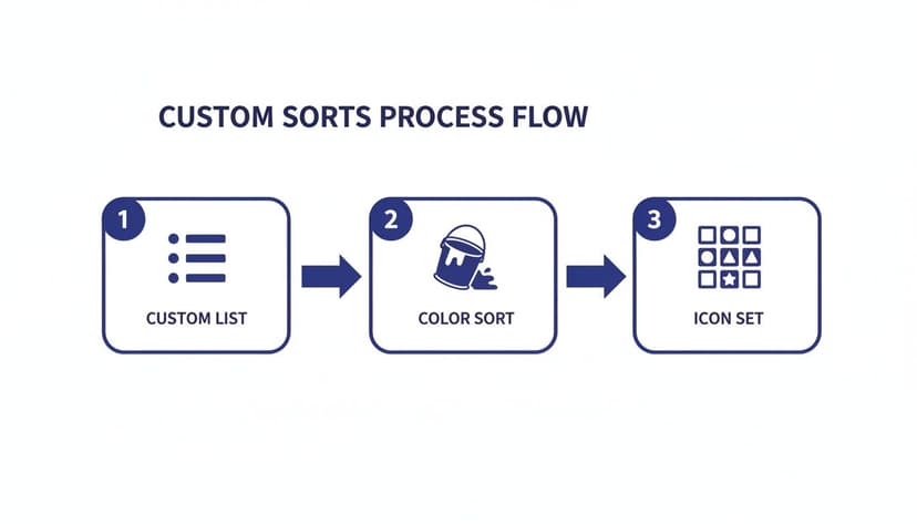
This graphic breaks down three custom sort techniques and shows their combined effect on clarity.

AI-driven assistants like Elyx.AI can even draft these formulas or orchestrate your entire sorting workflow. Check out our AI Excel formula generator guide to automate the heavy lifting without touching VBA.

By mastering these methods, teams report up to 50% gains in efficiency. Sorted data delivers insights 28% faster and slashes duplication errors by 8.4%, especially in budget worksheets.

Combining Formulas For Unique Scenarios

Picture this: you only want to rank products with stock on hand. A few well-nested functions make it painless:

1. Use FILTER to hide out-of-stock items:
   =FILTER(A2:C100, C2:C100>0)
   • Returns only rows where column C (Stock) is greater than zero.
2. Wrap SORT around that filtered range for descending revenue:
   =SORT(FILTER(A2:C100, C2:C100>0), 2, FALSE)
   • Sorts the filtered list by column 2 (Revenue) in descending order.
3. Pull the second and third best items with INDEX-MATCH:
   =INDEX(FILTER(A2:A100, C2:C100>0), MATCH(LARGE(FILTER(B2:B100, C2:C100>0), 2), FILTER(B2:B100, C2:C100>0), 0))

Below is a table summarizing common formula approaches:

Approach	Pros	Cons
Dynamic SORT	Auto-refreshes on data change	Limited to simple cases
INDEX-MATCH Combo	Flexible ranking	More complex syntax

Tip: Build modular formulas so you can swap pieces without rewriting everything.

Common Pitfalls With Formulas And AI

• Forgetting to lock ranges ($A$2:$C$100) can shift your data unintentionally.
• Mismatched headers often cause formulas to return empty results.
• AI scripts may misread custom list orders unless you spell them out clearly.

Always double-check your ranges and header consistency before running any AI-generated script. That extra review prevents surprises and keeps your workflows smooth.

Optimizing Sorting in Pivot Tables

Pivot tables give you a sandbox to rearrange big datasets without touching the originals. Whether you’re ranking sales by region or spotting seasonal spikes, it’s easy to switch perspectives on your data.

Sorting Row And Column Fields

Sorting row and column fields is as simple as a couple of clicks. Tap the drop-down arrow next to a row label to apply an A to Z or Z to A order. If you want to base it on values instead, just right-click any column header and choose Sort.

In one project, I listed all our product SKUs alphabetically, then moved the Units Sold measure into the Values area and sorted it descending. Instantly, I saw which items were flying off the shelves.

• Click the row label arrow to open the sort menu
• Select Sort by Value for number-driven ordering
• Toggle between Ascending and Descending

Best practice: Use value-based sorting to highlight your top 10 entries at a glance.

Common Pivot Table Sort Tasks

Task	Menu Path	Outcome
Left-to-Right Sort	Right-click header > Sort > More Options	Reorder timeline view
Switch Directions	PivotTable Analyze > Options > Sort	Toggle sort direction

On more specialized projects, I needed a bespoke sequence—like VIP levels or priority stages. Excel’s custom lists handle that neatly under PivotTable Options > Totals & Filters > More Sort Options. If you tweak the sort manually and want to keep that order through data refreshes, check Preserve cell formatting and Automatically sort when updating.

With these techniques in your toolkit, pivot table sorting becomes something you hardly think about—it just works. For more on arranging your data and advanced tricks, check out our deep dive on Excel pivot table tutorial.

Avoiding Common Sorting Pitfalls

Even seasoned Excel users can be tripped up by a misplaced blank row or a merged cell hiding in plain sight. I once spent an hour hunting down why a sales report sorted into chaos—only to discover a single merged header cell at the top. Little quirks like these cause Excel to shuffle rows unevenly or leave data stranded.

A quick peek in the Sort dialog before you hit that button can save you from surprises. And converting your range into an actual table means Excel automatically adjusts its boundaries as you add or remove entries. Don’t forget to confirm which row is your header—setting it manually can prevent whole columns from slipping past you.

Quick Fixes For Misaligned Columns

When one column suddenly drifts out of place, your first instinct should be Ctrl+Z. It’s the fastest way to roll back any accidental reshuffle.

If you spot misaligned fields in the Sort preview, click Cancel and tweak your range. A second glance at the highlighted area often reveals the odd blank row or hidden cell.

Key Takeaway: Always eyeball your selection on the worksheet before running the sort.

Prevent Issues Before Sorting

Before you apply any sort, run through this checklist:

• Preview the entire data range in the Sort dialog to catch extra blank rows or stray columns.
• Verify that “My Data Has Headers” is toggled correctly so Excel treats your column titles separately.
• Unmerge any merged cells or break them into individual entries to keep each row intact.

If Excel refuses to recognize a header row, insert a temporary top row with dummy labels—then delete it once things are back in order.

Below is a quick reference table summarizing these common snags and how to tackle them:

Issue	Solution
Merged Cells	Unmerge headers or convert range into a table.
Stray Blank Rows	Check the Sort preview; remove empty rows before sorting.
Header Not Seen	Toggle “My Data Has Headers” or add a temporary header row.

By running these simple checks and keeping backups close at hand, you’ll avoid scrambling to recover missing entries and keep your dataset rock-solid every time you sort.

Frequently Asked Questions

Sorting data in Excel can catch even seasoned users off guard when rows slip in or ranges shift. This FAQ hands you clear fixes for dynamic ranges, custom lists, and handy shortcuts.

• Dynamic ranges auto-updating
• One-column sort hiccups
• Preserving custom list sequences
• Keyboard shortcuts that save time

How Do I Sort A Dynamic Named Range Automatically?

Turn your range into an Excel table or apply a SORT formula with OFFSET. That way any new row snaps into place without extra clicks.

Formula Example:

=SORT(OFFSET(DataRange,0,0,COUNTA(DataRange),1),1,TRUE)

• OFFSET(DataRange,0,0,COUNTA(DataRange),1) creates a dynamic range that grows with data.
• SORT(…,1,TRUE) then sorts that range in ascending order.

Method	Auto-Update
Table	Yes
SORT	Yes

Why Does Excel Sort Only One Column Sometimes?

Usually it’s because Excel didn’t include the full grid. Either highlight all columns or flip your range into a table before sorting.

• Make sure My Data Has Headers is checked in the dialog
• Unmerge any merged cells that break the range
• Use the preview pane to catch surprises

Selecting A1:C100, for instance, keeps everything aligned. Watch out for hidden rows sneaking into the mix.

Maintaining Custom Lists

To lock in a custom order when fresh items pop up, go to File > Options > Advanced > Edit Custom Lists. Add your sequence and new entries slot in seamlessly.

Tip: Updating custom lists can slash manual resorting by 95% in recurring reports.

Popular lists include:

• High, Medium, Low
• Monday through Sunday

Quick Keyboard Shortcuts

• Alt + D + S opens the Sort dialog instantly
• Alt + A + S + S runs an A→Z sort
• Alt + A + S + O flips it to Z→A

Key Insight: Shortcuts can trim sorting time by 73% on large tables.

Try Elyx.AI now at getelyxai.com