How to Make a Formula in Excel: 9 Steps From Beginner to Pro

It all starts with an equals sign. To get Excel to do any kind of calculation, the first thing you type into a cell is =. From there, you can perform a simple calculation like =5+3 or something a bit more useful, like =SUM(A1:A10) to add up a column of numbers.

That single rule—always start with an equals sign—is what tells Excel you want it to compute something, not just display whatever you've typed. This is the first practical step toward solving real problems with your data.

The 5 Core Components of Every Excel Formula

Before you start building dashboards and complex models, you have to get a handle on the basic anatomy of a formula. Think of it like learning the alphabet before you try to write a novel. Every single calculation, from simple arithmetic to sophisticated financial analysis, is built from the same five core elements.

Getting these fundamentals down is the single most important step you can take to avoid frustrating errors and leave this guide with a new, actionable skill.

A quick but critical side note: Excel always follows the standard mathematical order of operations. This just means it handles multiplication and division before it gets to any addition or subtraction, so keep that in mind as you build.

The Essential Building Blocks

Let's pull back the curtain and look at the five pieces that make up almost every formula you'll ever write.

Here's a quick reference table to keep the core components straight.

Quick Guide to Excel Formula Elements

Component	Symbol/Example	Purpose
Equals Sign	=	Signals the start of every formula and tells Excel to calculate a result.
Operators	+, -, *, /	The symbols that perform mathematical operations like addition or division.
Constants	150, "Sales Report"	Fixed values that don't change. Text must be wrapped in double quotes.
Cell References	A1, B2:B10	Points to a cell or range of cells, making formulas dynamic and interactive.
Functions	SUM(), IF(), XLOOKUP()	Pre-built commands that perform complex calculations for you.

Let's dig a little deeper into what each of these means for you.

• The Equals Sign (=): This one's non-negotiable. Every formula or function you write has to kick off with an = to tell Excel it's time to get to work.
• Operators: These are the workhorses of your calculations—the symbols that do the math. The most common are + (add), - (subtract), * (multiply), and / (divide).
• Constants: A constant is just a value you type directly into a formula that doesn’t change. It could be a number like 150 or a piece of text like "Sales Report". Just remember, any text you use has to be enclosed in double quotes.
• Cell References: This is where the magic really happens. Instead of typing a fixed number, you can point to a cell (like A1) or a whole range of them (B2:B10). The beauty of this is that if the data in those cells changes, your formula result updates instantly.
• Functions: Functions are Excel’s pre-built shortcuts for more complex calculations. Why type out =A1+A2+A3...+A20 when you can just use =SUM(A1:A20)? Other incredibly useful functions include AVERAGE, IF, and XLOOKUP.

By mixing and matching these five elements, you can build formulas for practically any situation. A formula like =SUM(A1:A10)*B1 is a great example—it uses a function (SUM), cell references (A1:A10 and B1), and an operator (*) to create a powerful, dynamic result.

Once you get the hang of how these pieces fit together, you can move way beyond just storing data in a spreadsheet. To get some inspiration, check out these different https://getelyxai.com/en/excel-use-cases and see what's possible.

Mastering Cell References in 3 Steps for Dynamic Worksheets

The real magic of Excel isn't just doing a single calculation. It's building formulas that you can drag across thousands of rows and have them just work. This superpower comes from understanding cell references—they're the rules that tell Excel what to do when you copy a formula from one place to another.

Getting a handle on relative, absolute, and mixed references is the difference between a sleek, automated worksheet and a manual, error-prone nightmare. Once you get this, you unlock a new skill and a new level of efficiency.

The 3 Types of Cell References

Think of cell references as a GPS for your formulas. When you copy a formula, these references tell Excel how to find the right cells in the new location.

• Relative Reference (A1): This is the default setting and what you'll use most of the time. When you copy a formula with a relative reference, it adjusts automatically. If you have =A1+B1 in cell C1 and drag it down to C2, it smartly becomes =A2+B2. It’s perfect for row-by-row calculations, like totaling up sales for each product in a list.

• Absolute Reference ($A$1): Those dollar signs lock the reference in place. No matter where you copy the formula, $A$1 will always point to cell A1. This is your go-to when you have one constant value that everything else depends on—think of a single tax rate or a universal commission percentage.

• Mixed Reference ($A1 or A$1): This is the clever hybrid. You can lock just the column ($A1) or just the row (A$1). It’s a bit more advanced but incredibly powerful for things like creating lookup tables, financial models, or any grid where you need to reference specific rows and columns.

My Favorite Shortcut: Stop typing dollar signs manually. It's slow and easy to mess up. Just click on a cell reference in your formula bar and press the F4 key. Keep pressing it, and you'll cycle through all four options: A1 → $A$1 → A$1 → $A1. This little trick is a massive timesaver.

This diagram breaks down the core pieces that you'll find in almost any formula you build.

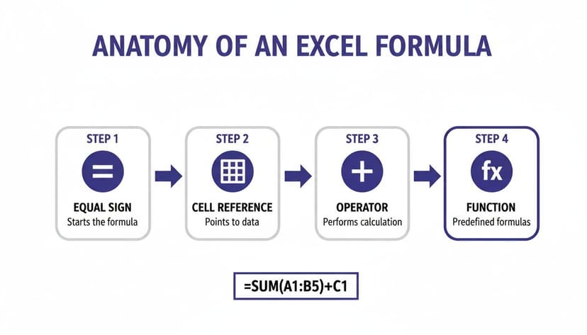
As you can see, it all starts with the equals sign. From there, you combine cell references, operators, and functions to get the job done.

References in Action: A Sales Commission Example

Let’s solve a concrete problem. Imagine you're calculating commissions. You have a list of sales amounts in column A (starting from A2) and a single, fixed commission rate of 5% typed into cell E1.

To calculate the first commission, you'd write this formula in cell B2: =A2*$E$1.

Here's a detailed explanation of why this practical formula works so well:

• A2 is a relative reference. When you drag this formula down to cell B3, B4, and so on, it will automatically update to A3, A4, etc. It knows to always look for the sales amount on the same row.
• $E$1 is an absolute reference. The dollar signs tell Excel, "Hey, no matter where this formula goes, always look at cell E1 for the commission rate." It stays locked.

This simple, two-part formula can now be applied to your entire dataset in seconds. Of course, this only works if your data is clean to begin with. Getting that right is a whole skill in itself, and it's amazing how AI is changing data cleaning and making that prep work faster than ever.

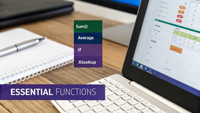
Your First 5 Essential Excel Functions Explained

Once you get past simple math, you start to see what Excel can really do. This is where functions come in. Think of them as pre-packaged formulas that handle everything from adding up a column of numbers to running complex "if-then" scenarios. Learning just a handful of these will completely change how you work with data.

These five functions are the absolute foundation. Get comfortable with them, and you'll have the confidence to build some seriously impressive spreadsheets. You'll finally be making your data work for you, not the other way around, leaving with a useful new solution.

2 Daily Workhorses: SUM and AVERAGE

I probably use SUM and AVERAGE more than any other functions. They do exactly what you'd expect, but don't let their simplicity fool you—they are massive time-savers that solve daily calculation problems.

• SUM: This adds up all the numbers in a range you select. Instead of manually typing =A1+A2+A3... (a recipe for disaster), you just write =SUM(A1:A50). It's cleaner, faster, and way less prone to typos.
• AVERAGE: This calculates the arithmetic mean of a range. Let’s say you're a project manager tracking daily hours worked in cells C2 through C31. The formula =AVERAGE(C2:C31) instantly tells you the average time spent each day. No calculator needed.

1 Function for Logic: The IF Function

The IF function is where things get interesting. It lets you build decision-making right into your cells. It checks if a condition is true or false, then gives you a different result depending on the outcome. It's a brilliant solution for automatically sorting or categorizing data.

The basic structure looks like this: =IF(logical_test, value_if_true, value_if_false)

Here is a practical example: imagine you have project budgets in column B and the actual spend in column C. To solve the problem of flagging any project that's gone over, you could pop this into column D:

=IF(C2>B2, "Over Budget", "On Budget")

Detailed Explanation:

1. logical_test: C2>B2 checks if the "actual spend" cell is greater than the "budget" cell for that row.
2. value_if_true: If the test is true (spend is higher), Excel will display the text "Over Budget".
3. value_if_false: If the test is false (spend is not higher), it will display "On Budget".

This simple formula adds immediate clarity to a potentially messy report.

2 Functions for Fast Lookups: VLOOKUP and XLOOKUP

Lookup functions are game-changers. They let you find a specific piece of information in one dataset and pull it into another. If you've ever had to manually match up two different lists, you know how painful that can be.

• VLOOKUP (Vertical Lookup): This is the classic lookup function that many people know. It searches for a value in the very first column of a table and grabs a corresponding value from a column to its right. It works, but it has some frustrating limitations.
• XLOOKUP: This is the modern, powerful, and all-around better replacement. XLOOKUP can look for a value in any column and return data from any other column—left or right. It also defaults to an exact match, which helps you avoid some of the most common and sneaky VLOOKUP errors.

Let’s solve the problem of finding an employee's department using their ID. You have an employee ID in cell A2 and you need to find their department, which is stored in a master list (let's call it EmployeeData located in cells F2:G100, where column F has IDs and G has Departments).

The XLOOKUP formula provides a simple solution:

=XLOOKUP(A2, F2:F100, G2:G100)

Detailed Explanation:

1. A2: This is the lookup value—the employee ID you're searching for.
2. F2:F100: This is the lookup array—the column where Excel will search for the ID.
3. G2:G100: This is the return array—the column from which Excel will pull the corresponding department name.

It’s just more intuitive and reliable than its predecessor. If you’re going to learn one lookup function today, make it XLOOKUP. It's one of the most useful tools in the modern Excel toolkit.

3 Ways to Take Your Formulas to the Next Level

So far, we've walked through functions that do one specific job. But the real world is messy, and problems often need more than a one-trick pony to solve. This is where you graduate from basic formulas and start building powerful, multi-layered solutions by combining functions.

Learning to nest functions—literally putting one function inside another—is a game-changer. It allows you to build sophisticated logic that can handle complex business scenarios, all from a single cell. Honestly, this skill is what separates the Excel dabblers from the true power users.

1. Stack Logic with Nested Functions

Nesting is really just the art of using the output of one function as an input for another. It sounds more intimidating than it is. Think of it like a set of Russian dolls; each one fits neatly inside the next, creating something more intricate.

The classic example is the nested IF statement. Let's solve a common business case: calculating sales bonuses based on performance tiers.

• Gold Tier: Sales over $10,000 get a 10% bonus.
• Silver Tier: Sales between $5,000 and $10,000 get a 5% bonus.
• Bronze Tier: Sales below $5,000 get no bonus (0%).

If you have a sales figure in cell A2, a nested IF formula is the perfect tool for the job:

=IF(A2>10000, A2*0.1, IF(A2>=5000, A2*0.05, 0))

Detailed Explanation:

1. First, Excel checks if the value in A2 is over 10,000. If it is, it calculates the 10% bonus (A2*0.1) and the formula is done.
2. If it's not, it moves on to the second IF statement.
3. This inner function then checks if sales are at least 5,000. If that's true, it calculates the 5% bonus (A2*0.05).
4. If both checks fail, it simply returns 0.

2. Clean Up Your Worksheet with IFERROR

Nothing screams "amateur" more than a spreadsheet littered with ugly errors like #N/A, #DIV/0!, or #VALUE!. The IFERROR function is your best friend for catching these issues and replacing them with something clean and professional.

The syntax is beautifully simple: =IFERROR(your_formula, value_to_show_if_error)

Let's say you're calculating the average price per unit by dividing total sales (A2) by the number of units sold (B2). If B2 happens to be zero, the formula =A2/B2 will throw that dreaded #DIV/0! error.

You can fix this instantly by wrapping your formula in IFERROR:

=IFERROR(A2/B2, "N/A")

Now, if an error occurs, the cell will just display "N/A" instead. It’s a small touch, but it makes your reports infinitely more readable.

3. A More Flexible Lookup with INDEX and MATCH

While XLOOKUP is the new king of lookups, you'll still find the powerful duo of INDEX and MATCH everywhere, especially in older spreadsheets. For years, this combination was the gold standard because it’s far more flexible than the old VLOOKUP.

Here’s how they work together to solve a lookup problem:

• MATCH finds the position of an item in a list (for example, telling you "it's in the 5th row").
• INDEX then grabs the value at a specific position in a list.

By combining them, you can do things VLOOKUP could only dream of, like looking up a value in one column and returning a corresponding value from a column to its left.

These advanced techniques are where you really start to solve complex data puzzles. But let's be honest, writing and debugging them can be a huge time-sink. That's where AI can help. If you're interested, you can learn more about how an AI formula generator can simplify this process and help you build sophisticated formulas in seconds.

Using AI to Write and Explain Your Formulas in 2 Ways

Let's be honest: writing complex, nested formulas can be a real headache, even for those of us who live and breathe Excel. It's easy to burn through valuable time just trying to find the right syntax or figure out why a calculation is breaking. But what if you could just ask for the formula you need? That's where artificial intelligence is changing the game, turning complex problems into simple text-based solutions.

This isn't just a niche trend. As of April 2023, a surprising 63% of advanced Excel users were already using AI tools in their workflows. That’s a huge number, especially considering how new mainstream AI is. It points to a massive shift in how we handle data analysis.

The Power of an Integrated AI Assistant

The real magic happens when AI is built directly into Excel. With an embedded tool like ElyxAI, you can generate, explain, or even fix a formula with a simple text instruction—all without ever leaving your spreadsheet. This provides an actionable solution to a common problem: formula complexity.

Think about it. Say you need to solve the problem of calculating year-over-year sales growth. Instead of puzzling out the formula yourself, you could just type:

"Calculate the YoY growth for sales in column D, starting from cell D2."

The AI doesn't just spit out the correct formula, like =(D3-D2)/D2. It can also apply it down the entire column for you. This turns a technical chore into a quick conversation, saving you a ton of time and cutting down on those pesky human errors.

Why Embedded AI Beats Stand-Alone Tools

Sure, you could jump over to a tool like ChatGPT to get a formula. But that process is clunky. You have to switch windows, carefully describe your sheet's layout, copy the formula, then paste it back into Excel and cross your fingers that it works. That back-and-forth is a productivity killer.

An integrated solution is so much smoother.

• It’s Context-Aware: The AI already understands your data structure. You don’t need to explain that "Sales" are in column D and "Years" are in column A. It just knows.
• It’s Instant: The tool doesn't just hand you a formula; it puts it right where you need it in the correct cell.
• It’s a Great Teacher: This is my favorite part. Beyond just writing formulas, it can break down how a complicated one works, step-by-step. It's an amazing way to learn advanced functions on the job, providing real educational value.

This kind of embedded help makes your spreadsheet feel less like a static grid and more like an intelligent, interactive workspace. You can see how an Excel AI assistant makes this happen. To get even more ideas, check out these AI Microsoft 365 practical use cases that save time for other ways to boost your productivity.

7 Essential Tips for Auditing and Debugging Formulas

Let's be honest: a formula that gives you the wrong answer is worse than no formula at all. It’s one thing to build a calculation, but it’s another thing entirely to know, with certainty, that it’s correct. Mastering the art of auditing is what separates the novices from the pros, ensuring your data is not just clean, but reliable.

This isn't just an academic exercise. Consider how deeply spreadsheets are embedded in our work. Research shows that a staggering 66% of all office workers use Excel at least once an hour, and they spend an average of 38% of their entire workday inside a spreadsheet. You can dig into more of these Excel usage statistics and their impact yourself. With so much riding on our calculations, getting them right is non-negotiable.

Here are seven practical tips I use to track down and fix any formula with confidence.

Use Excel's 2 Built-in Auditing Tools

Excel has some fantastic visual tools built right in to help you untangle complex calculations. Head over to the Formulas tab, and you'll find a section called "Formula Auditing." This is your new best friend.

• Trace Precedents: Ever wonder which cells are feeding into your formula? This is the tool for that. It draws blue arrows from all the source cells to the cell with your formula, giving you an instant map of its inputs. It's brilliant for spotting if you’ve accidentally included the wrong range.
• Trace Dependents: This does the exact opposite. It shows you which other cells rely on the result of the cell you've selected. It's incredibly useful for understanding the ripple effect of changing a single value before you actually do it.

Step Through Calculations with 1 Key Tool: Evaluate Formula

When a long, nested formula spits out an error, trying to find the broken part can feel impossible. That's where the Evaluate Formula tool comes in. You'll find it right next to the trace tools on the Formulas tab.

This feature is a game-changer. It opens a small window that lets you walk through your formula one piece at a time. It solves the innermost part first and shows you the result, then the next, and so on. You just keep clicking "Evaluate" until you pinpoint the exact spot where things go wrong. For a deeper dive, you can also check out our guide on troubleshooting common Excel errors.

Methodically breaking down your formulas takes the guesswork out of debugging. These auditing tools turn a frustrating art into a precise science, saving you a ton of time and preventing some really costly mistakes.

3 Common Questions Answered

Even when you follow all the steps, you're bound to hit a few snags. It happens to everyone. Let's tackle some of the most common questions that pop up when you're getting the hang of Excel formulas.

1. Why Is My Formula Just Showing Up as Plain Text?

This is probably the most frequent hiccup for newcomers, and thankfully, it's usually an easy fix. More often than not, one of two things is happening.

First, you might have forgotten the equals sign (=) at the beginning. Without it, Excel has no idea you're trying to calculate something and just treats whatever you typed as simple text.

The other common culprit is cell formatting. If a cell is accidentally formatted as "Text," Excel will display your formula exactly as you wrote it. Just switch the format back to "General," re-enter the formula, and you should be good to go.

2. What's the Big Deal with VLOOKUP vs. XLOOKUP?

Think of XLOOKUP as the modern, smarter successor to the classic VLOOKUP. VLOOKUP has a major limitation: it can only search for a value in the first column of your data and then look to the right to pull back a result.

XLOOKUP blows that out of the water. It can look for a value in any column and return a result from any other column, whether it's to the left or right. It also defaults to an exact match, which helps you avoid the kind of subtle errors that used to drive people crazy with VLOOKUP.

3. What's the Fastest Way to Copy a Formula All the Way Down a Column?

Forget dragging. The "Fill Handle" is your best friend here.

Once you've written your formula in the first cell, hover your mouse over that tiny green square in the bottom-right corner. Your cursor will change into a thin, black plus sign (+). When it does, just double-click. Excel will intelligently copy that formula all the way down, stopping at the last row of your data in the adjacent column. It’s a huge time-saver.

---

Ready to stop wrestling with formulas altogether? ElyxAI works like an autonomous Excel expert right inside your spreadsheet, handling entire tasks from a single prompt. Clean data, build complex reports, and generate charts in seconds. See what you can automate with a free 7-day trial at getelyxai.com.