8 Actionable Tips on How to Link Cells in Excel

Tired of the endless copy-paste cycle between Excel sheets, just hoping you didn’t miss anything? We've all been there. But what if you could connect your data so it updates automatically? That's exactly what linking cells does, and it's one of the most powerful, time-saving skills you can learn in Excel.

Figuring out how to link cells in Excel is your first step toward building smarter, more reliable spreadsheets that do the heavy lifting for you.

Why Bother Linking Cells? 4 Game-Changing Benefits

Let's be honest, manually updating data across multiple spreadsheets is a nightmare. It’s not just boring; it’s a massive risk. One forgotten update can throw off an entire report, mess up a financial forecast, or lead to some really bad business decisions.

When you link cells, you create a live connection. Change the original cell, and every single cell linked to it updates instantly. No fuss, no manual checks.

This one skill is the foundation of great spreadsheet design. It’s so crucial, in fact, that it’s considered one of the essential tools and techniques for business analysts for wrangling complex data. Linking turns your static, boring reports into dynamic dashboards and connects isolated islands of data into a single, cohesive system.

The 4 Big Wins: What Linking Actually Does for You

Once you get the hang of it, you’ll see the benefits immediately. Instead of juggling separate files, you start building an interconnected web of information that works together.

Here’s what you stand to gain:

• 1. Rock-Solid Consistency: Everyone works from the same numbers because there’s only one source. Say goodbye to version control headaches.
• 2. More Free Time: Think of all the time spent copying and pasting into summary sheets or dashboards. Linking automates that, freeing you up for more important work.
• 3. Fewer Human Errors: Manual data entry is prone to mistakes. Linking dramatically cuts down on the risk of typos and other slip-ups.
• 4. Live, Dynamic Reports: Build financial models and reports that refresh automatically as new information comes in.

Linking cells is like telling your spreadsheet how to update itself. You go from being a manual data entry clerk to an architect who designs an automated system. That's the real difference between a casual user and an Excel pro.

Ultimately, knowing how to link cells in Excel isn't just a neat trick—it's a strategic way to manage your data. It opens the door to a ton of advanced Excel use cases, from project management dashboards to slick sales trackers. This guide will walk you through everything you need to know.

7 Foundational Ways to Link Cells in Excel

Before you can build complex, dynamic spreadsheets, you have to get the basics down. Linking cells is the bedrock of making Excel work for you, and there are a handful of core methods every user should know. These techniques are the tools in your toolbox for everything from simple on-sheet summaries to pulling data across entire workbooks.

Let's walk through them, starting with the simplest and building our way up to more powerful approaches. Knowing which one to grab for a specific task is what separates the novices from the pros.

1. Direct Cell References: The Starting Point

The simplest link you can create is a direct cell reference. It's the first thing most of us learn. You just type an equals sign (=) in a cell, click another cell, and hit Enter. That's it.

For example, typing =A1 into cell B1 creates a live connection. Whatever you put in A1 will now instantly show up in B1. This is your bread and butter for quick calculations and summaries on the same worksheet. It's simple, but it's the foundation for almost every other linking method.

2. Linking Across Different Worksheets

Most real-world projects are bigger than a single sheet. You’ll often have a summary or dashboard tab that needs to pull key numbers from other tabs, like "Q1 Sales" or "Marketing Spend." This is where linking across sheets comes in.

The formula is pretty intuitive: =SheetName!CellAddress.

So, if you want your main "Dashboard" to show the grand total from cell F50 on your "Q1 Sales" sheet, you’d simply use the formula =‘Q1 Sales’!F50.

• Formula: =‘Q1 Sales’!F50
• Explanation: The single quotes (' ') are required because the sheet name "Q1 Sales" contains a space. The exclamation mark (!) tells Excel to look on the specified sheet. F50 is the cell address to pull data from.

Pro Tip: If your sheet name has a space in it, like "Q1 Sales," Excel automatically wraps the name in single quotes: ='Q1 Sales'!F50. Forgetting those quotes when typing manually is a common source of formula errors, so keep an eye out for that.

3. Connecting to Entirely Different Workbooks

Sometimes, your data isn't just on another sheet; it's in a completely different file. Think of a master financial report that consolidates numbers from separate budget and expense workbooks. To do this, you need to create an external link.

The syntax just adds the workbook name in square brackets: =[WorkbookName.xlsx]SheetName!CellAddress.

For instance, to link to cell B2 on "Sheet1" in a file called "SalesData.xlsx," the formula would be =[SalesData.xlsx]Sheet1!$B$2.

• Formula: =[SalesData.xlsx]Sheet1!$B$2
• Explanation: The workbook name [SalesData.xlsx] is enclosed in square brackets. Sheet1! specifies the worksheet, and $B$2 is the absolute reference to the cell. Excel uses an absolute reference (with $) so the link stays locked on that specific cell even if you drag the formula. If the source workbook is closed, Excel will helpfully add the full file path for you.

4. Using Paste Link for a Quick Connection

Honestly, typing out long file paths and sheet names is a pain and a surefire way to make a typo. For a much faster and error-proof way to link workbooks, just use Paste Link.

It couldn't be simpler:

1. Open both Excel files.
2. In the source file, copy the cell you want to link from (Ctrl+C).
3. Switch to your destination file, click where you want the link, and open the Paste Special menu (Alt+E+S).
4. Just click the Paste Link button in the bottom-left corner.

Excel does the heavy lifting and writes the perfectly formatted external link formula for you. It's my go-to for creating a few quick links without having to think about the syntax.

Choosing the right method can feel tricky at first. This quick decision tree helps visualize which path to take depending on where your data lives.

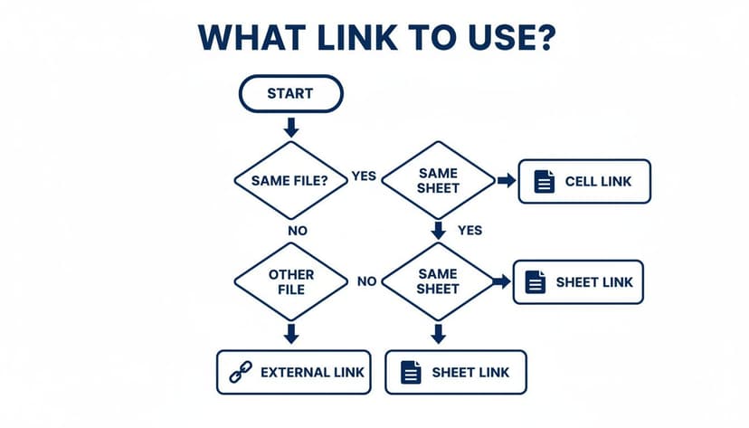
As you can see, it all starts with one question: is the data in the same workbook? From there, the choice becomes much clearer.

Comparison of 4 Core Excel Cell Linking Methods

To help you decide which manual method fits your needs, here’s a quick-glance table comparing the four most common approaches. Each has its own strengths and is designed for a particular job.

Linking Method	Best For	Example Formula	Key Advantage	Potential Drawback
Direct Reference	Simple calculations and summaries on the same sheet.	=A1	Fast, simple, and intuitive.	Limited to a single worksheet.
Cross-Sheet Link	Creating summary dashboards that pull data from other tabs.	=Sales!F50	Keeps workbooks organized and easy to navigate.	Sheet names with spaces require single quotes.
External Workbook	Consolidating data from multiple, separate Excel files.	=[Data.xlsx]Sheet1!$B$2	Connects disparate data sources into one view.	Links can break if source files are moved or renamed.
Paste Link	Quickly creating a few external links without manual typing.	(Generates External Link Formula)	Error-proof and requires no syntax memorization.	Less efficient for creating links in bulk.

This table makes it clear that there's a right tool for every task. For quick, on-sheet connections, a direct reference is perfect. But for building a comprehensive report from multiple files, you'll need the power of external links.

5. Leveraging Named Ranges for Cleaner Formulas

Let’s be real, a formula like ='Q4 Regional Sales'!$G$22 is hard to read and even harder to debug later. This is where Named Ranges come to the rescue. They let you give a simple, memorable name to a cell or a range of cells.

Instead of that cryptic reference, you could name cell G22 on the "Q4 Regional Sales" sheet TotalSales_Q4. Suddenly, your formula becomes =TotalSales_Q4. It's not just cleaner; it makes your entire spreadsheet more intuitive and easier for others (or your future self) to understand.

6. Aggregating Data with 3D References

What if you need to sum the same cell across a dozen different sheets? For example, adding up cell B5 from your "North," "South," "East," and "West" sales sheets. Writing a long formula like =North!B5+South!B5+East!B5+West!B5 is slow and clunky.

This is the perfect job for a 3D reference. It lets you perform a calculation across a continuous range of sheets.

The syntax looks like this: =FUNCTION(FirstSheet:LastSheet!CellAddress).

To solve our example, you would just use: =SUM(North:West!B5).

• Formula: =SUM(North:West!B5)
• Explanation: SUM is the function being applied. North:West defines the range of worksheets to include (every sheet between "North" and "West"). !B5 specifies the cell to sum on each of those sheets. This one clean formula grabs the value from cell B5 on every single sheet in the range. It’s incredibly efficient.

7. Speeding Things Up with an AI Formula Generator

Even with experience, remembering the exact syntax for every scenario can be a hassle. Thankfully, modern tools are here to help. If you need a complex formula but don't want to get bogged down in the rules, an AI formula generator is a fantastic assistant.

You can just describe what you need in plain English—like "Sum cell B5 from Sheet1 through Sheet4"—and the tool will generate the correct =SUM(Sheet1:Sheet4!B5) formula for you. It's a great way to bridge the gap between knowing what you want to accomplish and knowing the exact syntax to get it done.

4 Advanced Ways to Create Dynamic Links with Formulas

Once you've got the basics down, you can start building spreadsheets that are truly dynamic and intelligent. We're moving beyond simple, static connections and into formulas that create interactive, flexible links. This is where you can build reports and dashboards that respond to user input and even pull in live data from the web.

Let’s dive into four powerful formula techniques that will completely change how you work with data in Excel.

1. Build Clickable Navigation with HYPERLINK

A standard cell link pulls data from another cell, but the HYPERLINK function does something different: it creates a clickable link that takes you somewhere. This is a fantastic tool for building a table of contents on a summary sheet, guiding users to specific report sections, or linking out to a website directly from your spreadsheet.

The syntax is pretty simple: =HYPERLINK(link_location, [friendly_name])

• link_location: This is the destination path. It can be a web URL, a file path, or a reference to another cell in the same workbook (like "#Sheet2!A1").
• friendly_name: This is the text you want people to actually see and click on, such as "Go to Sales Data."

Imagine you have a massive workbook with dozens of different tabs. You can set up a "Table of Contents" sheet where each item is a clickable link. To create a link that jumps to cell A1 on a sheet named "Q3_Forecast," you’d use this formula:

• Formula: =HYPERLINK("#Q3_Forecast!A1", "View Q3 Forecast")
• Explanation: The # symbol indicates an internal link within the current workbook. "Q3_Forecast!A1" is the specific destination. "View Q3 Forecast" is the user-friendly text that will appear in the cell as a clickable link. One click, and your user is instantly transported to the right spot, making complex files so much easier to navigate.

2. Create Flexible References with INDIRECT

The INDIRECT function is easily one of Excel's most powerful tools for dynamic linking. It's a bit of a mind-bender at first: it takes a text string and tells Excel to treat it as a real cell reference. This lets you build your cell references on the fly using text from other cells or the results of other formulas.

The syntax is straightforward: =INDIRECT(ref_text, [a1])

• ref_text: A text string that looks like a cell reference (e.g., "Sheet2!B5") or a cell containing that text.
• a1: This is optional. TRUE means use A1 style (the default), while FALSE is for R1C1 style.

Here’s a classic real-world example. Say you're building a financial model to compare monthly sales. Each month's data lives on its own sheet ("Jan," "Feb," "Mar," etc.). Instead of manually updating your summary formulas every time you want to see a different month, you can use INDIRECT.

First, create a dropdown list in cell A1 with the month names. Then, use this formula to pull the total sales figure from cell G50 of whichever sheet is selected:

• Formula: =INDIRECT("'" & A1 & "'!G50")
• Explanation: A1 refers to the cell with your dropdown list. The & operator joins text together. The formula constructs a text string like 'Feb'!G50 based on the value in A1. INDIRECT then converts that text string into a live reference, pulling the data from the correct sheet. This lets you build a highly interactive report with a single formula. If you want to get more comfortable with functions like this, our guide to essential Excel formulas is a great place to start.

The INDIRECT function is a game-changer for building flexible dashboards. It lets you create models where the user can select what data they see, all without you ever needing to edit a single formula.

3. Pull in Real-Time Data with Linked Data Types

Modern Excel, especially in Microsoft 365, has a killer feature called Linked Data Types. This isn't just a link to another cell; it's a live connection to a massive online database like Bing. It allows you to pull structured, real-time information right into your spreadsheet.

It’s surprisingly easy to use.

• Type a company's name, like "Microsoft," into a cell.
• Go to the Data tab and click Stocks in the Data Types gallery.
• Excel converts that text into a data-rich object linked to live stock info. You can then pull specific details with simple formulas, like =A1.[Price].
  • Formula: =A1.[Price]
  • Explanation: Assuming cell A1 has been converted to the "Stocks" data type for Microsoft, this formula extracts the current stock price. The .[Price] part is called an "extractor" and can be used to pull dozens of data points like "Market Cap," "52-week high," etc.

This works for stocks, currencies, geographic locations, and more. It transforms your spreadsheet from a static document into something that breathes, constantly updated with information from the outside world. You can read more about what linked data types are available in Excel on Microsoft's support page.

4. Experiment with AI-Powered Functions

The next frontier for data linking involves putting artificial intelligence right into the formula bar. Microsoft is rolling out new functions that let you "talk" to large language models without ever leaving your spreadsheet.

This evolution is significant. Since Excel 365 introduced linked data types in 2016, professionals have gained access to real-time, Bing-powered data. This has been a massive time-saver for tasks requiring external information.

Newer AI functions, like the experimental COPILOT function, are taking things to another level. With this, you can write a natural language prompt as part of a formula and get an AI-generated response directly in a cell. For example, you could reference a column of customer feedback and use a formula to ask an AI to classify the sentiment of each comment. This is a whole new kind of "linking"—connecting your cell not just to data, but to an intelligent service that can analyze it for you on the fly.

3 Essential Tips for Managing and Fixing Broken Excel Links

Linking cells and workbooks in Excel is fantastic for building dynamic reports that update automatically. But let's be real—the real headache isn't creating the links; it's keeping them from breaking. A broken link can silently wreck your data, leading to bad reports and even worse decisions.

That's why knowing how to troubleshoot these connections is just as crucial as knowing how to create them. All it takes is one renamed file or a deleted cell to set off a chain reaction of errors, turning your beautifully crafted model into a mess.

1. Finding and Fixing External Links

Ever inherited a complex workbook and had no idea where all the data was coming from? Your first move should always be to hunt down any external connections. Excel actually gives you a handy dashboard for this.

Just head over to the Data tab and click on Edit Links. This little dialog box is your mission control for managing every external source file.

From here, you can do a few key things:

• Check Status: Get a quick health check to see if Excel can find the source file.
• Update Values: Manually pull in the latest data from one or all of the linked files.
• Change Source: If a file was moved or renamed, you can easily point the link to its new location here.
• Break Link: This severs the connection completely, turning the cell’s formula into a static value.

A quick word of warning: Break Link is a one-way street. Once you break it, the formula is gone for good. You can't undo it, so be absolutely sure before you click.

2. What to Do About the Dreaded #REF! Error

Nothing strikes fear into the heart of an Excel user quite like a spreadsheet filled with #REF! errors. This error is Excel’s way of screaming that a formula’s reference is gone. When it comes to linked cells, it usually boils down to a few common culprits.

Figuring out the "why" is half the battle. Most of the time, the problem is one of these:

• A Deleted Source: The link is pointing to a cell, row, column, or even an entire worksheet that no longer exists.
• A Moved or Renamed File: The workbook your link depends on was moved to a new folder or someone changed its name.
• A Bad Copy-Paste Job: You copied a formula with relative references, and now it's pointing to a location that doesn’t make sense.

To fix it, you’ll need to do a bit of detective work. Click the cell with the error and look at the formula bar. If you see a file path that looks wrong, use the Edit Links dialog to point it to the right place. If it’s an internal link, you might have to trace it back to the source sheet to see what's missing and then adjust your formula. If you're running into other issues, our guide on how to handle common Excel errors can help.

3. Taking Control of Security and Update Pop-Ups

Every time you open an Excel file with external links, you get that familiar security pop-up asking if you want to update them. It’s a useful safety net, but it can also be annoying. The good news is you can control how Excel handles this.

You can tweak these settings by going to File > Options > Trust Center > Trust Center Settings > External Content. Here, you can tell Excel exactly how to manage links to other workbooks—whether to always ask, disable them quietly, or just enable them automatically.

This isn't just about convenience; it's a serious governance issue in many companies. Proper link management is a high-stakes game, especially when managing critical financial or risk data. For a deeper dive into best practices, this detailed guide to data linking provides excellent insights.

Automating Cell Linking with AI in Excel

Linking cells in Excel is incredibly useful, but let's be honest—it can be a real grind. When you're trying to pull data from dozens of different sheets or workbooks, the process becomes a tedious, click-heavy marathon. It's a recipe for mistakes. One wrong cell reference, and you've got a cascade of errors on your hands.

This is exactly where AI tools built for Excel, like Elyx, are making a huge difference. Instead of you being the one to manually build every single link, you simply tell the AI what you want to accomplish.

The old way was all about syntax and precision. The new way is a conversation.

From Tedious Clicks to Simple Commands

Picture this common scenario: you need to build a master dashboard that summarizes total sales from 20 different regional worksheets. Doing this by hand is a nightmare. You'd have to jump into each sheet, locate the correct "total" cell, and painstakingly create each link back to your summary page, double-checking everything as you go.

With an AI agent integrated into your spreadsheet, the process looks completely different. You just type a straightforward command, like you're talking to a colleague:

"Link the total sales from each regional sheet to my summary dashboard."

The AI gets to work immediately. It understands what you're asking, finds the right data across all those sheets, and builds all the necessary formulas for you. It handles the monotonous mechanics, freeing you up from the grunt work.

The AI Edge: Speed and Flawless Accuracy

The difference between the old manual way and this new AI-powered approach is night and day, especially as your spreadsheets get more complex. This isn't just about saving a bit of time; it's about eliminating huge chunks of manual labor and sidestepping the human errors that inevitably creep in.

Here's what you gain:

• Serious Time Savings: A task that might have taken you an hour of meticulous linking can now be done in seconds with a single command.
• Near-Zero Errors: AI doesn't get tired and click the wrong cell or make a typo in a formula. Your data consolidation is accurate from the get-go.
• Focus on Insights, Not Formulas: You can finally concentrate on the bigger picture—analyzing the data—instead of getting bogged down in the technical weeds of how to connect it all.

This shift is really the future of working in Excel. You define the "what," and the AI figures out the "how." For anyone who manages complex data and wants to escape the tedious parts of the job, checking out an AI assistant for Excel can be a massive productivity win. It turns daunting tasks into simple conversations.

Wrapping It Up: Becoming an Excel Linking Pro

We’ve covered a lot of ground, haven't we? From a simple =Sheet1!A1 reference to more complex formulas and even bringing AI into the mix. The big idea here is that linking cells in Excel is so much more than just pulling data from one place to another. It's about building smarter, more dynamic spreadsheets that practically run themselves.

Think about it: once you get the hang of these methods, you're not just saving time on data entry. You're creating powerful, automated reports and dashboards while slashing the risk of manual errors. My advice? Don't try to master everything at once. Start with the basics and begin weaving the more advanced tricks into your daily work as you get comfortable.

And when you hit a wall with a particularly messy or large-scale linking task, remember that modern tools are ready to step in. They can be a huge help, taking care of the tedious mechanics so you can focus on what the data actually means.

For those who need to manage truly complex data systems or want to offload the heavy lifting, an Excel and Sheets Virtual Assistant can offer that next level of expert support. They live and breathe this stuff, handling advanced linking and troubleshooting so you don't have to.

You've got the toolkit now. The real magic happens when you start applying these skills to your own projects. Go turn those static spreadsheets into the interconnected, data-driven powerhouses they're meant to be.

3 Common Questions About Linking Cells in Excel

Once you start linking cells, especially between different workbooks, a few common questions tend to pop up. Let's tackle some of the most frequent hurdles you might encounter so you can solve them quickly.

1. How Do I Stop My Links From Breaking When I Move Files?

This is probably the most common headache with external links. The simplest, most effective way to avoid broken links is to keep your source and destination files together in the same folder. When you move that folder as a complete unit, Excel is smart enough to keep the relative paths intact.

If you absolutely have to move the files separately, you'll need to give Excel the new address. Just head over to the Data tab, click Edit Links, and point the formula to the file's new home. For shared projects, I highly recommend using a cloud service like SharePoint or OneDrive. They manage file paths much more elegantly than a local network drive, which can save your whole team a lot of frustration.

2. What’s the Real Difference Between a Direct Link and Paste Link?

At the end of the day, both methods create the exact same formula, something like =[Workbook.xlsx]Sheet1!$A$1. The difference is all in the how.

Typing a link directly gives you full control from the get-go. It’s perfect when you know exactly what you want to write.

Paste Link, on the other hand, is a fantastic shortcut. You just copy a cell (Ctrl+C), then use the Paste Special menu (Alt+E+S+L) to drop the link in. I find Paste Link is much faster for creating a single, specific link. But if you need to create a whole series of links down a column, manually typing the first one and dragging the fill handle is usually more efficient.

3. Can I Get Updated Values Without Opening the Source File?

Yes, you can, but there's a catch you need to be aware of. When you open a workbook containing external links, Excel will ask if you want to update them. If you click 'Update', it will pull the last saved value from the closed source file.

Here's the important part: this is a snapshot, not a live feed. It's only as current as the last time the source file was saved. To get true, real-time data reflecting the very latest changes, the source workbook must be open.

If you need automated refreshes from closed files on a schedule, you'll have to step up to a more powerful tool like Power Query.

---

Tired of wrestling with manual Excel tasks? Imagine an AI colleague working inside your spreadsheet, handling everything from data cleanup to report building with simple instructions. That's what Elyx AI does.

Give it a try with a free 7-day trial and see how much time you can get back. Experience the future of spreadsheets at getelyxai.com.