How to Filter Data in Excel From Basics to Advanced Tricks

Filtering data in Excel is a fundamental skill for turning a mountain of information into something you can actually use. It lets you temporarily hide the rows you don't need, so you can focus on what matters. The fastest way to get started is with AutoFilter, a simple tool that adds drop-down arrows to your column headers, letting you instantly pick and choose the data you want to see.

Your Starting Point for Filtering Data in Excel

Staring at a massive spreadsheet can be intimidating. Thankfully, Excel has a whole toolkit designed to bring clarity to your data. Filtering isn't just about hiding rows—it's about asking specific questions and getting immediate answers right there in your sheet. Whether you're a financial analyst combing through quarterly expenses or a project manager checking on task deadlines, knowing how to filter is a core skill that makes your job easier and your decisions smarter.

Most people start with AutoFilter, but the options go much further. For example, you might need to see all sales records from the "West" region. That’s a perfect job for a quick filter. But what if you need a list that automatically updates whenever a new sale is logged for that region? That’s where a modern dynamic array function like FILTER() really shines.

Choosing the Right Filtering Method

Which tool should you grab? It really depends on what you're trying to accomplish. Are you doing a quick, one-and-done check, or are you building a dashboard that needs to stay current? Knowing your options is the first step to working more efficiently.

• For quick, static tasks, AutoFilter is your go-to. It’s fast, simple, and gets the job done.
• For dynamic, live lists, the FILTER() function is the modern powerhouse. It creates a spill range that reflects changes in your source data instantly.
• For visual, interactive reports, Slicers and PivotTables are fantastic. They let you (and others) explore data with simple clicks, no formulas required.

This decision tree gives you a great visual roadmap for picking the right method for your specific task.

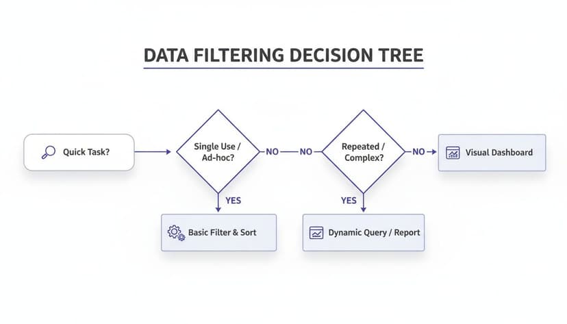
As the flowchart shows, simple tasks are perfect for basic filters, but if you need your results to be dynamic or highly visual, you'll want to reach for the more advanced tools. It's a handy reference for any analysis.

Excel has come a long way since AutoFilter first arrived, a feature that boosted productivity by an estimated 30% for data review tasks. Today, modern tools like the FILTER() function can slash manual sorting and filtering time by up to 70% on large datasets.

To help you choose quickly, here's a simple breakdown of the main filtering methods and where they work best.

Choosing the Right Excel Filter Method

Filter Method	Best For	Key Feature
AutoFilter	Quick, simple filtering on one or more columns.	Easy to apply with one click; intuitive drop-down menus.
Custom Filter	Applying specific conditions like "greater than" or "begins with".	More control than the basic checklist for text, numbers, and dates.
FILTER() Function	Creating dynamic, separate lists that update automatically.	A modern array formula that "spills" results into a new range.
Advanced Filter	Complex criteria involving AND/OR logic across multiple columns.	Can extract a unique list of records to a different location.
PivotTables & Slicers	Interactive data summarization and exploration.	Slicers provide user-friendly buttons to filter PivotTable data visually.
Power Query	Filtering large datasets from multiple sources before they load into Excel.	Handles millions of rows and performs complex transformations.

Each method has its place, and knowing which one to use for the right situation is what separates the casual user from the power user.

Of course, none of these filters will work correctly if your data is a mess. A crucial first step is always to make sure your data is clean and well-structured. For a complete walkthrough on this, check out our guide on how to clean data in Excel. Tidy data ensures your filters are reliable and saves you from frustrating troubleshooting later on. Don't skip this foundational step.

Mastering Everyday Filtering with AutoFilter

If there’s one workhorse feature in Excel, it’s AutoFilter. For day-to-day data tasks, it's the quickest and most straightforward way to cut through the noise in a large dataset. The moment you apply it, those little drop-down arrows appear on your column headers, instantly turning a static spreadsheet into an interactive tool.

My go-to shortcut to get started is Ctrl+Shift+L. Just click anywhere inside your data, hit that combo, and you're ready to start exploring.

The real beauty of AutoFilter isn't just checking and unchecking boxes, though. It’s designed to answer more complex questions, helping you turn raw information into actual insights. Think of it as your first stop whenever you need to get a quick handle on what a dataset is telling you.

Going Beyond Basic Checkboxes

While picking values from the list is handy for simple tasks, you'll get so much more done by diving into the custom filters. These built-in options let you apply specific rules to your data, which is where things get really powerful.

Imagine you're looking at a project plan. Instead of manually scanning dates, you can use a custom date filter to instantly see all tasks with a deadline that falls "within the last quarter" or "is after" today. It’s a lifesaver for flagging overdue items without the manual headache.

Text filters are just as useful. If you're sifting through customer feedback, you could filter a comments column for any text that "contains" the word "excellent" to pull up positive reviews. Or, you could look for the word "bug" to isolate technical problems that need attention.

Filtering Numbers and Dates with Precision

Excel gives numbers and dates their own set of specialized filters, and this is where you can uncover some really useful trends, especially in sales or financial data.

• Top 10 Items: Need to find your best-performing products or top salespeople? Just filter your revenue column for the "Top 10" values. You can even tweak this to show the top 10% or any other number you want.
• Above/Below Average: This one is brilliant. You can instantly see which data points are outliers by filtering for values "Above Average" or "Below Average." Excel figures out the average for that column on the fly.
• Date Ranges: Forget manually selecting date ranges. Use dynamic filters like "This Week," "Next Month," or "Year to Date." They automatically update based on today’s date, so your report is always current.

I see a lot of people overlook these built-in operators. They'll spend ages sorting and manually selecting rows when a simple "Greater Than" or "Does Not Contain" filter would have given them the answer in seconds.

Combining Filters for Pinpoint Accuracy

This is where AutoFilter really shines—when you start layering filters across multiple columns. Each filter you add refines the results from the previous one, letting you zero in on exactly what you need with incredible precision.

Let's say you run an e-commerce store and you're analyzing customer reviews. You could apply a multi-column filter to get a very specific answer:

1. First, filter the 'Product Line' column to show only "Electronics."
2. Then, on the 'Rating' column, filter for values equal to "5."
3. Finally, add a date filter to the 'Submission Date' column to see only reviews from "This Year."

With just three clicks, you've gone from a massive table to a clean list of all five-star reviews for electronic products submitted this year. This is the essence of how to filter data in Excel for real, actionable insights.

One thing to watch out for, though, is that precise filtering can expose data quality problems. You might notice the same customer review showing up multiple times, for instance. Before doing any serious analysis, it’s always a good idea to clean up your dataset first. You can learn more about this in our guide on how to remove duplicate rows in Excel, which will help ensure your filtered results are both accurate and unique.

When You Need More Firepower: Solving Complex Scenarios with Advanced Filter

AutoFilter is your go-to for most day-to-day filtering tasks, but what happens when the questions you're asking your data get more complicated? That's when you bring out the big guns: Advanced Filter. It’s the tool you need when your filtering logic involves complex OR conditions across different columns, something the standard filter just can't handle.

Let's say you're pulling together a targeted marketing list. You want to find every customer who is either from Texas OR has spent over $1,000, regardless of their state. With AutoFilter, this is a non-starter. You could easily find Texas customers who have also spent over $1,000 (a classic AND condition), but you can't isolate those two independent rules. Advanced Filter was built for exactly this kind of problem.

The secret sauce behind Advanced Filter is its criteria range—a small, separate area on your worksheet where you lay out the rules of the game. This simple but brilliant approach keeps your filtering logic separate from your data, making it incredibly easy to build, check, and tweak complex queries without messing with the original table.

Setting Up a Criteria Range for Complex Logic

First things first, you need to build this criteria range. It’s pretty straightforward: just copy the exact column headers you want to filter by and paste them into an empty spot on your sheet. The real magic is in how you arrange the criteria underneath those headers.

• For AND Logic: When you place criteria in the same row, you're telling Excel to find records that meet all of those conditions. For instance, putting "Texas" under a State header and ">1000" under a Sales header in the same row will find only the customers from Texas who spent over $1,000.
• For OR Logic: This is where it gets interesting. Placing criteria in different rows tells Excel to find records that meet any of those conditions. This is the key to cracking our marketing list puzzle.

Let’s go back to that marketing list. In your criteria range, you’d put "Texas" under the State header. Then, on the very next row down, you’d put ">1000" under the Sales header. This setup tells Excel, "Show me every row where the State is Texas OR the Sales amount is greater than 1000." Simple as that.

The ability to define multi-row OR conditions is what makes Advanced Filter so powerful. It transforms your filtering from a simple checklist into a robust query tool, allowing you to extract precisely the dataset you need for analysis or reporting.

This feature allows users to pull records based on complex conditions that basic AutoFilter just can't touch. In fact, some companies have found it can cut data processing times by as much as 50%. For tasks like sales analysis, these custom filters can reveal demographic insights 35% faster. You can dig into even more details about these filtering capabilities on Microsoft's official site.

Extracting Unique Values and Copying Results

Advanced Filter has another fantastic trick up its sleeve: extracting unique values from a list. Got a column with thousands of repeating entries, like customer names or product categories, and just need a clean, distinct list? Advanced Filter can pull that for you in seconds. You just have to check the "Unique records only" box in the dialog.

Even better, it can copy the filtered results to a brand-new location, either on the same sheet or a different one entirely. This is a massive win for reporting. Instead of filtering your main table "in-place" and then fumbling with copy-pasting the visible cells, you can generate a clean, standalone report of your results, leaving your source data completely untouched.

This feature is crucial for preserving the integrity of your original dataset. For even more robust data extraction and transformation workflows, many pros eventually move on to more specialized tools. To learn about one of the most powerful options available right inside Excel, check out our complete Excel Power Query tutorial.

Creating Dynamic Reports with the FILTER Function

If you’ve been using Excel for a while, you’re probably familiar with AutoFilter and maybe even the Advanced Filter. They’re great for quick, in-place data exploration. But modern Excel has something far more powerful up its sleeve: the FILTER function. This is a true game-changer. It creates a live list that updates automatically as your source data changes. No more re-applying filters every time something gets updated.

At its core, FILTER is beautifully simple. You only need two things to get it working: the array (the full range of data you want to filter) and the include argument (the rule or condition you want to apply). The result is a brand-new, separate table with just the data that meets your criteria.

Your First Dynamic Filter Formula

Let's walk through a real-world example. Say you have a project management tracker with tasks listed in columns A through C. Column C tracks the status: "Complete," "In Progress," or "Not Started." If you want to create a live list of all completed projects, the formula is incredibly straightforward.

You'd just type this into a blank cell:
=FILTER(A2:C50, C2:C50="Complete")

Let's quickly break that down:

• A2:C50 is our array—the entire list of tasks.
• C2:C50="Complete" is the include part. This tells Excel to look down the status column and only pull rows where the value is "Complete."

The moment you hit Enter, the formula "spills" all the matching results into a new range. Best of all, if you go back to your original data and change another task's status to "Complete," it instantly pops up in your filtered list.

Handling Multiple Conditions with Ease

The FILTER function really starts to shine when you need to layer on multiple conditions. You can combine criteria using a simple multiplication (*) for AND logic (both things must be true) or an addition (+) for OR logic (either thing can be true).

Imagine you need to find all tasks for the "Marketing" department (column B) that are also marked as "High Priority" (column D).

Here’s how you’d build that formula:
=FILTER(A2:D100, (B2:B100="Marketing") * (D2:D100="High Priority"))

That little * acts as the AND operator, making sure a row only gets pulled if both conditions are met. This feels so much more intuitive than messing around with the clunky criteria ranges required by the old Advanced Filter.

Combining FILTER with Other Dynamic Functions

This is where things get really interesting. You can nest FILTER inside other powerful functions like SORT and UNIQUE to refine your results without any extra steps. It’s all done in a single, elegant formula.

Let’s say you need an alphabetized list of unique salespeople who hit their quarterly target of over $50,000.

You can do it all in one go:
=SORT(UNIQUE(FILTER(A2:A100, B2:B100>50000)))

Here’s how Excel thinks through this one-liner:

1. FILTER: First, it grabs all salespeople from column A whose sales in column B are over 50,000.
2. UNIQUE: Next, it takes that list and instantly strips out any duplicate names.
3. SORT: Finally, it sorts the clean, unique list alphabetically.

One formula delivers a perfect report that stays up-to-date automatically. When formulas get this complex, I sometimes use an AI-powered Excel formula builder to help construct them on the fly, which saves a ton of time.

Here’s what a live FILTER looks like in a spreadsheet.

You can see how the formula in cell F5 is pulling data from the main table (A4:D18) based on the "East" region, creating that dynamic spill range.

Customizing for No Results

One little snag you might hit is the #CALC! error, which pops up when your filter doesn't find any matching data. Luckily, the FILTER function has a built-in fix. The optional third argument, [if_empty], lets you display a friendly message instead of an ugly error.

For example:
=FILTER(A2:C50, C2:C50="Overdue", "No Overdue Tasks Found")

Now, if there are no overdue tasks, the cell will just say "No Overdue Tasks Found." It's a small touch that makes your reports look much more professional.

Introduced with Microsoft 365, the FILTER function and its dynamic array capabilities were a massive leap forward. For many common reporting tasks, it can slash refresh times by an estimated 65% compared to old-school VBA macros.

Of course, Excel’s power doesn’t stop at filtering. Once you have your data, you’ll want to perform calculations and gain deeper insights. To do that, you'll need to master Excel formulas for accurate calculations and build more complex models.

Building Interactive Dashboards with Slicers

Static reports are often ignored. To create data presentations that colleagues and clients will actually use, you need to build dynamic, user-friendly dashboards that encourage exploration. This is where Slicers are a game-changer. They replace clunky dropdown filter menus with clean, visual buttons that anyone—regardless of their Excel skills—can use with confidence.

Instead of explaining how to use a filter, you can simply provide a dashboard with Slicers. This small change makes a significant difference, allowing users to focus on the insights they can uncover with a simple click rather than the mechanics of filtering.

Connecting Slicers to Your Data

You can connect Slicers to a formatted Excel Table or a PivotTable. The setup is straightforward: click anywhere inside your data, navigate to the Table Design or PivotTable Analyze tab in the ribbon, and select "Insert Slicer." A window will appear with your column headers. Just check the boxes for the fields you want to filter by, and the Slicers will appear on your worksheet.

Imagine you're working with a sales dataset. You could add Slicers for 'Region' and 'Product Category.' Now, anyone viewing the report can click the "North" button to see all sales for that area, then click "Electronics" to drill down further. The data filters instantly, and any linked charts or PivotTables update in real time.

Slicers are more than just a filtering tool; they're a communication tool. They make your data accessible and your reports feel incredibly professional, empowering people to answer their own questions without needing to ask you.

Visualizing Time with Timelines

If your dataset involves dates—and most do—there's a special type of Slicer you'll love: the Timeline. It’s a visually intuitive filter built specifically for date fields. Instead of a list of buttons, it gives you an interactive, scrollable timeline that makes analyzing data over time a breeze.

To add one, just select your Table or PivotTable, go to the design tab, and choose "Insert Timeline."

Once a Timeline is on your sheet, you can:

• Filter by different time periods: Jump between Years, Quarters, Months, or even Days with a single click.
• Drag to select a custom range: Want to see what happened in the last six weeks? Just click and drag the handles on the timeline to isolate that specific period.
• Spot trends quickly: It's so much easier to see seasonal patterns or monthly performance when you can visually slide through the data.

Pairing Slicers and Timelines is a powerhouse combination for any dashboard. A sales manager could use a Region Slicer to pick their territory and then use a Timeline to see how sales trended month-over-month last quarter. This is how to filter data in Excel in a way that truly tells a story and keeps your audience engaged.

Using AI for Smarter Data Filtering

Complex formulas and multi-step filtering can be challenging. But what if you could just ask Excel for the data you need? This is where artificial intelligence comes in, transforming how we interact with spreadsheets. We are moving from memorizing syntax and navigating menus to using simple, conversational commands.

This is not a future concept; it's available now with tools like Elyx.AI. By integrating directly into Excel, it allows you to filter large datasets by typing what you want in plain English. The focus shifts from the how of filtering to the what, enabling you to ask important questions about your data directly.

Natural Language Filtering in Action

Imagine a large sales report. You need to find a specific slice of information quickly. Traditionally, this would involve setting up number, text, and date filters—a multi-step process.

With an AI function like =ELYX.AI(), you can bypass these steps. You simply ask for what you need in one command.

For instance, to see all sales from California over $500 last month, you could type this formula into a cell:
=ELYX.AI("Show me all sales over $500 in California from last month from my sales data")

The AI interprets the request, understanding the multiple conditions—location, sales amount, and time frame—and instantly provides a clean, filtered list. The complex logic is handled behind the scenes, saving you time and reducing the risk of errors. This is a practical example of how you can use AI in Excel to automate your daily tasks.

The real magic of AI-driven filtering is its knack for understanding context. It can decipher what you actually mean, even if your request isn't perfect, and can clean up messy data on the fly. It makes tough analysis feel easy.

AI-Powered Data Cleaning During Filtering

AI's capabilities extend to cleaning data as it filters. Real-world datasets are often imperfect, containing typos, inconsistencies, and formatting issues that can disrupt analysis. AI can identify and correct these problems during the filtering process.

It acts as an integrated data-cleaning assistant:

• Standardizing Text: If your data contains "CA," "Calif.," and "California" in the same column, the AI recognizes them as the same entity and includes them all in the filtered results.
• Correcting Typos: It can identify and fix common misspellings in product names or customer details, ensuring no important data is excluded.
• Harmonizing Formats: AI can handle different date formats or currencies without requiring manual cleanup first.

This intelligent processing ensures the filtered data you receive is not only accurate but also consistent. Exploring different AI data analysis tools can help you spend less time on data preparation and more time uncovering valuable insights.

Troubleshooting Common Excel Filtering Problems

Even experienced Excel users can encounter filtering issues. These problems can be frustrating, but the solutions are usually straightforward. Let's review some of the most common challenges and how to resolve them.

Why Is My Filter Option Grayed Out?

This is a frequent problem where the Filter button on the Data tab is disabled. In most cases, the cause is one of two simple issues.

First, check if your worksheet is protected. Navigate to the Review tab on the ribbon. If you see an Unprotect Sheet button, click it and enter a password if required. This should enable the filter option.

If the sheet isn't protected, look at your sheet tabs at the bottom. If more than one tab is highlighted white, your sheets are grouped. Excel does not allow filtering across grouped sheets. To fix this, right-click on any of the grouped tabs and select Ungroup Sheets.

How Do I Work With Filtered Data?

Once your data is filtered, you need to manage the visible information effectively. Here are a few essential techniques for working with filtered data.

• Finding Blank Cells: To identify rows with missing information, click a filter dropdown arrow, uncheck "(Select All)," scroll to the bottom of the list, and check the box for (Blanks). This isolates all incomplete records for review.

• Copying Only What You See: A common mistake is using Ctrl+C on a filtered range, which copies hidden rows as well. To avoid this, first select your filtered data, then press Alt+; (Alt plus semicolon). This action selects only the visible cells. Now, when you press Ctrl+C, you will only copy the data you can see.

• Clearing All Filters in One Go: Instead of removing filters from each column individually, you can clear them all at once. Go to the Data tab and click the Clear button in the "Sort & Filter" group. The keyboard shortcut for this is Alt, A, C.

---

Ready to stop wrestling with complex filters and start getting answers in seconds? With Elyx.AI, you can filter, clean, and analyze your data using simple English commands. Discover a smarter way to work in Excel by visiting https://getelyxai.com and see how AI can transform your productivity.