Master the excel formula for difference: Top 9 Uses

A manager asks for a variance report. The file looks simple. Two columns, two periods, one deadline.

Then the key question shows up. Do they want the raw numeric gap, the signed change, the percent change, the absolute variance, the elapsed days, or a matched comparison between two tables? In Excel, difference isn't one thing. It's a family of calculations, and choosing the wrong one changes the story your report tells.

That’s why the best excel formula for difference depends on the business question first, not the syntax first. Sales teams care about growth direction. Finance teams often need neutral comparisons. Operations teams may need date gaps. Analysts working across messy files need lookup-based variance, not plain subtraction.

Your 9 Essential Excel Formulas for Calculating Differences

A common approach is to start with subtraction and stop there. That works for basic variance, but it breaks down fast once your workbook moves beyond a clean before-and-after table.

The practical toolkit usually includes these 9 formulas or formula patterns:

1. =B2-A2 for raw directional difference
2. =ABS(B2-A2) for magnitude only
3. =(B2-A2)/A2 for standard percentage change
4. =ABS(B2-B3)/AVERAGE(B2:B3) for symmetrical percentage difference
5. =B2-A2 when the cells are dates and you need days
6. =DATEDIF(start,end,"unit") for full years, months, or days
7. =YEARFRAC(start,end,basis) for financial time fractions
8. =SUMIFS(...) - SUMIFS(...) for conditional aggregated differences
9. =current_value - XLOOKUP(...) for matched row-by-row differences across tables

That list covers most reporting work you’ll run into in Excel. If you're comparing software options or looking for broader spreadsheet software for team workflows, it helps to understand which platform supports these formulas cleanly and which one adds automation on top.

Practical rule: Start by asking, “What exactly am I comparing?” Then ask, “Do I care about direction, magnitude, percentage, time, or matched records?”

The fastest analysts don’t memorize formulas in isolation. They map each one to a reporting problem. Monthly sales variance needs one approach. Supplier price comparison needs another. Employee tenure needs a different one again.

That’s the lens that makes the excel formula for difference useful instead of mechanical.

3 Foundational Formulas for Everyday Analysis

The basic excel formula for difference starts with subtraction. That sounds obvious, but most reporting mistakes happen because someone uses subtraction when they needed absolute variance or percentage change.

According to this explanation of Excel difference formulas, the subtraction operator =A1-B1 forms the cornerstone of Excel-based numerical analysis and supports work like KPI monitoring, budget variance tracking, and project reporting. That matches how analysts use it in day-to-day files.

Use subtraction when direction matters

If Q1 sales are in A2 and Q2 sales are in B2, use:

=B2-A2

This tells you whether the result moved up or down. A positive result signals an increase. A negative result signals a decline. That sign matters in finance, sales, and operations because it shows direction immediately.

A common mistake is flipping the order. If you want later minus earlier, write the formula that way every time. Consistency matters more than elegance.

Here’s a quick decision view:

Reporting need	Formula	Why it works
Month-to-month sales variance	=B2-A2	Keeps the sign
Budget vs actual gap	=Actual-Budget	Shows over or under
Inventory movement	=Current-Prior	Tracks change direction

If you want extra help building formulas from plain-English logic, this guide on how to make a formula in Excel is a useful reference.

Use ABS when only the size matters

Sometimes direction creates noise. If you’re measuring how far actual values deviate from target, you may only care about the size of the miss.

Use:

=ABS(B2-A2)

ABS removes the sign and returns a non-negative result. That makes it useful for tolerance checks, reconciliation work, and exception summaries.

If the business question is “how far apart are these values,” ABS is usually right. If the question is “did this go up or down,” ABS hides useful information.

Use percentage change when scale matters

A raw difference alone can mislead. A change of 50 means something very different on a base of 100 than on a base of 10,000.

Use:

=(B2-A2)/A2

This gives standard percentage change relative to the starting value. In the same sales example, it tells you not just the gap, but the size of that gap relative to Q1.

A quick walkthrough helps:

• B2-A2 calculates the raw change
• /A2 anchors that change to the old value
• Format as Percentage to make the result readable

Later in the article, the percentage section covers the cases where this formula is not the right one.

A short demo can help if you want to see the mechanics on screen:

Calculating Symmetrical vs Standard Percentage Change

Analysts often use percentage formulas as if they were interchangeable. They aren’t. The denominator decides what story the result tells.

Standard percentage change for before-and-after reporting

When you have a clear baseline, use standard percentage change:

=(New-Old)/Old

This is the right choice for month-over-month sales, cost increases from a prior contract, or revenue movement across reporting periods. One value comes first in time. The other comes later. The old value is the anchor.

That works because the question is directional. You want to know how much growth or decline occurred relative to where you started.

Symmetrical percentage difference for neutral comparisons

When neither value should dominate the comparison, use the symmetrical method:

=ABS(B4-B5)/AVERAGE(B4:B5)

As explained in Acuity Training’s breakdown of percentage difference in Excel, this formula divides the absolute difference by the average of the two values, which treats both values equally. That makes it a better fit when you’re comparing peer values such as two supplier quotes, two business units, or two campaign results without a natural “old” and “new.”

This distinction matters in real reporting. If you compare supplier A to supplier B with standard percentage change, the result changes depending on which supplier you put in the denominator. That can create avoidable debates in meetings.

Use standard percentage change for timeline analysis. Use symmetrical percentage difference for side-by-side comparison.

A simple comparison table

Scenario	Better formula	Why
This month vs last month sales	=(New-Old)/Old	There is a baseline
Old price list vs new price list	=(New-Old)/Old	One list replaces the other
Supplier A vs Supplier B	=ABS(A-B)/AVERAGE(A:B)	Neither is the base
Team North vs Team South output	=ABS(A-B)/AVERAGE(A:B)	Neutral comparison

One more practical issue shows up in financial models. If the old value is zero, standard percentage change can produce a division error. In those cases, analysts usually add logic such as IF or IFERROR so the report displays a readable outcome instead of breaking the sheet.

If your work includes growth rates over longer periods, this article on the CAGR formula in Excel is a useful companion because CAGR solves a related but different problem.

2 Smart Ways to Calculate Date and Time Differences

Dates look simple in Excel until someone asks for tenure in complete years, elapsed months, or a fractional year for accrual logic. Then plain subtraction stops being enough.

Use subtraction for day counts

If A2 is a start date and B2 is an end date, this works:

=B2-A2

Excel stores dates as serial values, so subtraction returns the number of days between them. That’s enough for many operational tasks like delivery lead time, days overdue, or days between request and completion.

It’s also the cleanest option when your report only needs elapsed days. Don’t overcomplicate it.

Use DATEDIF for complete units

DATEDIF is better when the business question needs complete years, months, or days rather than a raw day count.

Examples:

• =DATEDIF(A2,B2,"y") for full years
• =DATEDIF(A2,B2,"m") for full months
• =DATEDIF(A2,B2,"d") for total days

This is useful for employee tenure, customer relationship age, contract duration, or age calculations. It gives the kind of output people expect when they ask, “How long has this person been here?”

A few cautions make it more reliable:

• Check date order. Start date should come first.
• Use real Excel dates. Text that looks like a date can break the result.
• Match the unit to the question. Full months and total days are not interchangeable.

For a more detailed walkthrough, this DATEDIF function guide is handy.

Most date errors come from one of two issues: the cells contain text instead of dates, or the analyst used day subtraction when the stakeholder wanted full months or years.

Use YEARFRAC for finance and prorating

YEARFRAC solves a different problem. It calculates the fraction of a year between two dates.

Use:

=YEARFRAC(A2,B2,basis)

This matters in finance when you need to prorate annual values such as revenue recognition, interest, or depreciation over part of a year. A simple day count can be informative, but it doesn’t express the result in the form many financial models need.

Here’s where each one fits best:

Need	Formula	Best use
Exact elapsed days	=B2-A2	Operations and scheduling
Complete years or months	=DATEDIF(...)	HR and tenure reporting
Fraction of a year	=YEARFRAC(...)	Financial models

Time differences need the same discipline

The same logic applies to times. If one cell contains a start time and another contains an end time, subtraction works when the values are stored properly. Then formatting decides whether the result is readable.

If you see strange decimals, the formula usually isn’t wrong. The formatting is.

Advanced Conditional and Lookup-Based Differences

Real reports rarely compare two cells sitting next to each other. More often, you need to compare filtered totals or matched records pulled from separate tables.

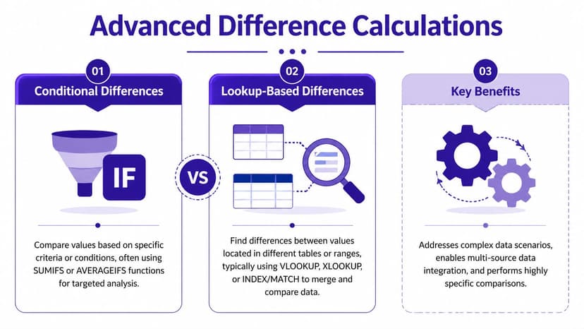
SUMIFS for conditional aggregated differences

Use SUMIFS when the difference you need depends on criteria. A common example is comparing sales totals for the same product across two regions.

Example:

=SUMIFS(sales_range,product_range,"Product A",region_range,"North")-SUMIFS(sales_range,product_range,"Product A",region_range,"South")

This formula doesn’t compare single records. It compares filtered aggregates. That’s a major difference.

Use it when you need questions like:

• Regional variance between North and South
• Target vs actual for one product line
• Department spend differences under matching conditions

XLOOKUP for matched row-by-row differences

Use XLOOKUP when your values live in separate tables and need to be matched by an ID, SKU, employee number, or account code.

Example:

=B2-XLOOKUP(A2,old_id_range,old_price_range,"Not Found")

This compares the current value in B2 to the matching historical value returned from another table. It’s a strong pattern for price changes, roster updates, and comparing old and new exports from different systems.

If you want a deeper reference, this XLOOKUP function resource is worth keeping nearby.

Which one to choose

Situation	Better tool	Reason
Compare total sales for one region vs another	SUMIFS	You need filtered totals
Compare each current SKU price to prior list	XLOOKUP	You need matched records
Compare actual hours by team and month	SUMIFS	Criteria drive the total
Compare employee salary across two exports	XLOOKUP	IDs drive the match

The trade-off is straightforward. SUMIFS is better for grouped business questions. XLOOKUP is better for one-to-one record comparison.

Field note: If you find yourself manually filtering a table, copying a number, then subtracting another filtered number, that’s usually a sign the job should move into SUMIFS.

One warning matters here. Lookup-based differences only work if your matching key is clean. Extra spaces, inconsistent IDs, or duplicate records can produce wrong differences that look perfectly reasonable. Those are the most dangerous errors because the formula returns something, just not the right thing.

Finding Rolling and Period-Over-Period Differences

Period-over-period analysis is where simple formulas start to feel either efficient or painful, depending on how the workbook is built.

A basic monthly trend report might list months in column A and values in column B. The classic formula in C3 is:

=B3-B2

Then you fill it down. That works, and for many static reports it’s still fine.

The helper-column method

The helper-column approach is familiar because it’s easy to audit. Anyone opening the file can inspect one row and understand the logic immediately.

It’s a good fit when:

• The report is fixed and won’t expand often
• The audience reviews formulas manually
• You need quick month-over-month or week-over-week variance

The downside is maintenance. Once people insert rows, paste over formulas, or extend the dataset inconsistently, the report starts drifting.

Dynamic arrays for modern rolling calculations

In modern Excel, dynamic arrays make rolling differences cleaner. If your values are in B2:B13, you can calculate the full sequence with:

=B3:B13-B2:B12

Excel spills the results down automatically. You don’t need to drag the formula row by row.

That changes how a dashboard behaves. Add new source rows, update the ranges, and the difference output updates as one expression instead of a patchwork of copied formulas.

Why this matters in live reporting

Rolling differences are rarely the end result. They feed trend charts, management packs, KPI summaries, and commentary. The cleaner the logic, the easier it is to trust the output.

Here’s the practical contrast:

Approach	Strength	Weakness
Fill-down helper column	Easy to inspect	Easy to break manually
Dynamic array subtraction	Cleaner and faster	Requires modern Excel habits

A common reporting pattern uses both. Analysts may build a dynamic calculation for the live dashboard, then keep a simpler helper-column version in a review tab for auditability.

The formula choice here isn’t about sophistication. It’s about how often the file changes, who maintains it, and how much manual editing the workbook will survive.

Troubleshooting 2 Common Issues and Automating with AI

A difference formula can be mathematically correct and still fail in a live report.

I see this in two situations more than any other. The first is circular data, where 359° and 1° are only 2 degrees apart, but standard subtraction returns 358. The second is exception handling, where one bad lookup or zero baseline pushes #N/A or #DIV/0! across a dashboard.

Angular differences are not standard subtraction

Angular data needs its own logic. Bearings, wind direction, machine rotation, and route headings wrap at 360 degrees, so the business question is usually "what is the shortest gap?" rather than "what is A minus B?"

As discussed in this engineering forum thread on polar degree calculations, the formula for the shortest angular difference is:

=MIN(MOD(A1-B1+360,360), MOD(B1-A1+360,360))

Use this when a normal variance formula would overstate movement because of the 0/360 boundary. In operations or logistics reporting, that distinction changes the conclusion. A vehicle heading shift of 2 degrees should not be reported as 358.

Error handling protects the report, not just the formula

The second issue is less about math and more about report design. A percentage difference formula may be fine, but if the baseline is zero or a lookup key is missing, the output becomes unreadable for everyone downstream.

A practical example:

=IFERROR((B2-A2)/A2,"N/A")

IFERROR does not solve the source problem. It gives finance, ops, or leadership a usable report while you decide whether the right fallback is "N/A", 0, or a custom message.

Use these checks before you trust the output:

• Use IFERROR when the audience needs readable exceptions
• Check the denominator before calculating percentage change
• Validate lookup keys before using lookup-based variances in summaries
• Separate circular measurements from ordinary numeric differences

That last point matters more than it looks. Sales variance, budget deltas, and inventory movement can share one pattern. Sensor angles and directional data cannot.

Where AI actually helps

Analysts rarely struggle with subtraction itself. The time drain is the repeated setup around it. Cleaning imported values, spotting zero denominators, fixing mismatched keys, filling formulas down, and rebuilding the same variance logic in a new workbook every week.

That is where an AI assistant like ElyxAI fits the process well. Instead of only suggesting a formula, it can help execute the surrounding spreadsheet work that usually takes longer than the formula choice itself. If you want a broader view of AI tools used across repeated business processes, this comprehensive AI workflow guide is useful context.

For Excel-specific use cases, this article on automating repetitive Excel reporting tasks shows where automation starts saving time. In practice, the win is consistency. The same rules for difference calculations, exception handling, cleanup, and formatting get applied the same way each cycle.

If you want Excel to do more than suggest formulas, Elyx AI is built for that. It works inside Excel, understands plain-language requests, and executes multi-step spreadsheet workflows, from cleaning data and calculating differences to building pivots, charts, and formatted reports.