CAGR Formula in Excel: 5 Ways to Calculate Annual Growth

You’re probably looking at a workbook right now with a start value, an end value, and a boss or client who wants “annual growth” in one clean number.

That’s where the cagr formula in excel earns its keep. It gives you a smoothed yearly growth rate that’s much more useful than eyeballing a trend line or averaging raw changes. And once you know the right method, it’s quick to calculate.

The catch is that Excel doesn’t give you one single dedicated CAGR button. You can calculate it manually, use built-in functions like RRI, RATE, and GEOMEAN, or switch to XIRR when your data is messy and real life refuses to fit neat annual periods.

Why Simple Averages Fail and CAGR Succeeds

A simple average feels tempting because it’s easy. You take a set of yearly changes, average them, and move on. But that shortcut often gives the wrong story.

In business reporting, growth usually compounds. Revenue, portfolio values, and customer counts don’t reset every year. Each year builds on the last one. A simple average ignores that compounding effect, which is exactly why stakeholders can walk away with a distorted view of performance.

CAGR, or compound annual growth rate, fixes that. It answers a more useful question: what constant annual rate would take you from the beginning value to the ending value over the full period?

Practical rule: If you need one number to summarize growth across multiple periods, use CAGR, not a plain average.

That distinction matters in board decks, budget reviews, and investment analysis. It’s one reason many Financial Analysts rely on CAGR when comparing performance over time. They need a metric that reflects compounding, not just arithmetic smoothing.

If you’re fuzzy on how a regular average works in Excel, this quick guide to the AVERAGE function is useful because it makes the contrast clearer. Average is great for many tasks. It’s just not the right tool for compound growth.

What CAGR tells you

CAGR is best when you have:

• A clear start and end point. For example, first-year revenue and latest-year revenue.
• A multi-period comparison. It helps when one period had an unusual spike or dip.
• A need for one summary rate. Executives usually want one annualized figure they can compare across products, markets, or funds.

Where people get confused

Two things trip people up fast:

1. They confuse average yearly change with annualized compounded growth.
2. They treat uneven data like neat yearly data.

The first problem makes the result misleading. The second breaks the method entirely. Both are common, and both are fixable once you know which Excel formula fits the data you have.

The Classic CAGR Formula and its POWER Upgrade

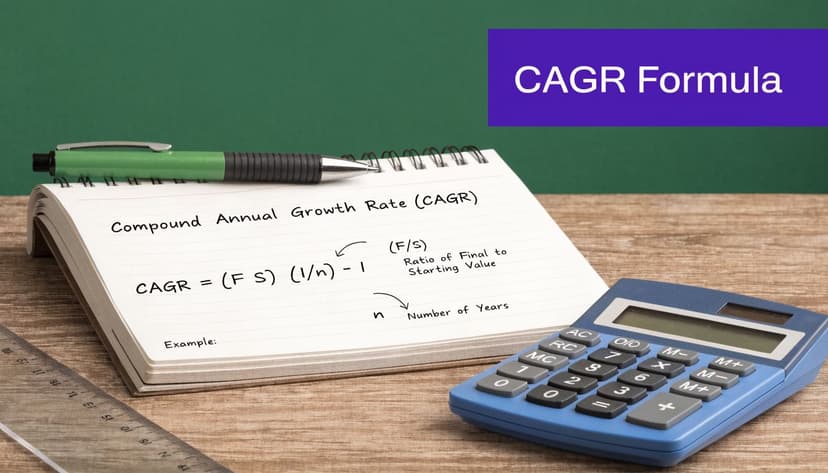
The standard cagr formula in excel is:

=(End Value / Start Value)^(1 / Number of Periods) – 1

That formula turns raw start and end values into an annualized growth rate. A worked example from Macabacus on calculating CAGR in Excel shows that an investment growing from $1,000 in 2021 to $1,330 in 2024 over 3 periods produces a 9.97% CAGR with =(1330/1000)^(1/3)-1.

How the formula works

Break it into pieces:

• End Value / Start Value gives the total growth multiple.
• 1 / Number of Periods converts that total growth into an annualized exponent.
• Minus 1 converts the growth factor into a rate.

If your years are in A2:A5 and your values are in B2:B5, a practical version is:

=(B5/B2)^(1/(YEAR(A5)-YEAR(A2)))-1

Format the result as a percentage and Excel will show the annual rate in a way people can read quickly.

Why this method is still worth learning

Manual CAGR is still the foundation because it teaches the logic. If you don’t understand the math underneath, it’s much easier to misuse a built-in function later.

It’s also flexible. You can drop cell references into dashboards, financial models, and summary sheets without needing a special function. When I audit someone else’s workbook, this is often the easiest version to read first.

If your data is clean and evenly spaced, the manual formula is usually the clearest option.

A cleaner version with POWER

The caret operator ^ works fine, but some people find it harder to read in nested formulas. Excel’s POWER function makes the exponent piece more explicit:

=POWER(B5/B2,1/(YEAR(A5)-YEAR(A2)))-1

That does the same thing. It just reads more like plain English: take the ratio and raise it to the annualizing power.

If you want a quick reference for the syntax, this guide to the POWER function in Excel is handy.

When to choose manual formula versus POWER

Use the classic formula when:

• you want the most common version analysts recognize
• you’re teaching the concept
• you want compact formulas in a report tab

Use POWER when:

• Readability matters. Teams can parse it faster in shared models.
• You’re nesting formulas. Explicit functions are often easier to audit than operators.
• You prefer consistency. Some finance teams standardize on function-based formulas.

Both methods are valid. Neither is more “correct.” The better choice is the one your team can read, trust, and maintain.

3 Built-In Functions for Faster Calculations

Once you understand the manual formula, Excel’s built-in functions can save time. They also reduce the chance of parenthesis mistakes, which is one of the most common reasons CAGR formulas go wrong.

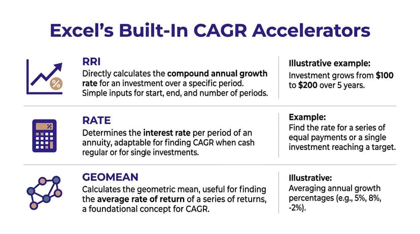
RRI for direct CAGR

If you want the closest thing to a built-in CAGR function, use RRI.

According to FormulaShq’s explanation of the RRI function, =RRI(nper, pv, fv) returns the compound annual growth rate directly, and an investment moving from $100 to $147 over 5 years returns 8%, which matches =(147/100)^(1/5)-1.

Example syntax:

=RRI(5,100,147)

Excel returns the rate as a decimal, so you’ll usually format the cell as a percentage.

RRI is great when your data is simple: beginning value, ending value, and evenly spaced periods.

RATE for finance-style models

RATE is more general. It’s built for interest rate calculations, but you can adapt it to CAGR by setting the periodic payment to zero.

Typical structure:

=RATE(nper,0,-pv,fv)

The important detail is the sign convention. The present value usually goes in as negative because it represents an outflow. That’s where many users slip.

RATE is useful when your workbook already uses finance functions and you want consistency across loan, investment, and return calculations.

GEOMEAN for a series of growth factors

GEOMEAN is different. It isn’t based on just a start and end value. It’s useful when you already have a sequence of annual growth factors and want the geometric mean.

That makes it a strong option for year-by-year return series. If your worksheet contains growth multipliers such as 1 + yearly return, GEOMEAN gives you the compounded average rate.

A guide to the GEOMEAN function in Excel is useful if you work with return series rather than endpoint values.

Excel Functions for CAGR at a Glance

Function	Syntax	Best For
RRI	=RRI(nper,pv,fv)	Direct CAGR from start, end, and periods
RATE	=RATE(nper,0,-pv,fv)	Financial models that already use rate-based functions
GEOMEAN	=GEOMEAN(range)-1	Series of annual growth factors or returns

Which one should you pick

Here’s the practical version I’d use in day-to-day work:

• Choose RRI when you want the quickest built-in answer.
• Choose RATE when your workbook is already structured like a financial model.
• Choose GEOMEAN when your data is a chain of yearly returns, not just one start and one end value.

Use the function that matches your data structure, not the one that looks most elegant.

That’s the shortcut. Most Excel mistakes happen because people force one formula onto the wrong shape of data.

Handling Irregular Dates and Cash Flows with XIRR

Most CAGR examples online assume life is tidy. One starting investment. One ending value. Nice even annual periods.

Real workbooks rarely look like that.

You may have one investment in March, another in September, a withdrawal later, and a final valuation at year-end. Standard CAGR methods don’t handle that timing properly.

Microsoft recommends XIRR for irregular cash flows and non-annual periods, and its guidance on CAGR in Excel notes that using standard CAGR in those situations can produce 20-30% calculation errors.

Why normal CAGR fails here

The classic formula assumes each period is equal. That’s fine for clean yearly data. It breaks when cash arrives or leaves on irregular dates.

If two cash flows happen far apart within the same year, plain CAGR treats them as if they happened on the same schedule. That’s the distortion.

How to structure XIRR correctly

Set up two columns:

• One column for cash flow amounts
• One column for the exact dates

Then use:

=XIRR(values,dates)

So if your cash flows are in B2:B10 and dates are in A2:A10, the formula is:

=XIRR(B2:B10,A2:A10)

You need at least one negative value and one positive value. That sign pattern tells Excel there was an outflow and an inflow.

If you want a refresher on syntax and practical setups, this guide to the XIRR function in Excel is a useful reference.

Where XIRR earns its place

Use XIRR when you’re dealing with:

• Interim deposits or withdrawals in investment tracking
• Project funding rounds that happened on different dates
• Irregular business cash flows instead of clean annual snapshots
• Monthly or uneven timing where annual period assumptions would mislead

Here’s a walkthrough that helps visually if you prefer to see the setup in action:

Standard CAGR is for endpoints across even periods. XIRR is for dated cash flows.

That’s the decision rule. If dates matter, use XIRR.

4 Common CAGR Pitfalls and How to Avoid Them

A CAGR formula can be mathematically correct and still give you a useless result if the inputs are wrong. Most errors come from data quality, period counting, or using the wrong function for the job.

Pitfall 1 with zero or negative values

CAGR formulas can throw #NUM! or #DIV/0! when the beginning or ending values are zero or invalid for the math. A practical fix highlighted in ExcelJet’s CAGR examples is to wrap the formula with IFERROR, such as =IFERROR((B7/B2)^(1/5)-1, "Invalid").

That doesn’t solve bad data, but it does stop ugly errors from spreading across a report.

Pitfall 2 with the wrong number of periods

This one is sneaky. People count rows instead of completed periods.

If your data runs from one year to another year, the number of periods is the gap between them, not the number of labels on the screen. Using the wrong n changes the annualized rate immediately.

Pitfall 3 with non-annual data

Quarterly and monthly data need care. If you use a yearly formula on non-annual periods without adjustment, you’re mixing time units.

Use a period count that matches the data frequency. If your timing is irregular enough that period math becomes awkward, that’s usually a sign you should move to XIRR.

Pitfall 4 with weak validation

Most tutorials stop at “here’s the formula.” In real files, validation matters just as much.

A stronger setup includes checks like these:

• Catch bad inputs early with IFERROR or IF.
• Verify start values before building dashboards.
• Check date order so your first and last periods are correct.
• Label invalid cases clearly instead of returning raw Excel errors.

A robust version might look like this:

=IFERROR((B7/B2)^(1/5)-1,"Invalid")

That’s not fancy. It’s professional.

Automate All CAGR Calculations in Seconds with ElyxAI

Knowing the formulas is still worth it. You need that judgment to choose between manual CAGR, RRI, RATE, GEOMEAN, and XIRR.

But in live reporting, the slow part usually isn’t the math. It’s the mechanics. Finding the right range, checking whether the dates are regular, copying formulas down, formatting outputs, and making sure the workbook doesn’t break when new data lands.

That’s where automation changes the workflow. Microsoft benchmark figures cited in this advanced Excel CAGR automation video state that using functions like RRI, RATE, and XIRR in automated workflows can reach 98% success rates versus 72% for manual formulas.

What that looks like in practice

Inside Excel, you can describe the task in plain English instead of building every step by hand. A request might be as simple as:

• Calculate CAGR for a selected revenue column
• Use XIRR if the date intervals are irregular
• Format the output as percentages
• Flag invalid rows where zeros or broken inputs appear

That approach is especially helpful if your work doesn’t stop at one formula. Many analysts also need summaries, commentary, and polished outputs for decision-makers. If that’s part of your process, this piece on AI report writing is a helpful companion because it focuses on turning analysis into finished business communication.

Why the AI route makes sense

The main gain isn’t just speed. It’s fewer avoidable clicks and fewer formula mistakes.

If you want Excel to execute the work instead of merely suggesting what to type, tools built for that job are worth a look. ElyxAI fits that model inside the spreadsheet itself, and you can see how the workflow works on the ElyxAI Excel AI page.

---

If you want Excel to calculate CAGR, detect irregular cash flows, clean errors, and format the result without the manual grind, try Elyx AI. It works directly inside Excel, so you can type what you need in plain English and let the add-in handle the spreadsheet work for you.