Master the Amortization Excel Formula: A Practical Guide

Calculating loan amortization in Excel is a powerful skill, and it primarily relies on three core functions: PMT, PPMT, and IPMT. Once you understand how these work together, you can build a detailed schedule that shows exactly how each payment reduces your debt and builds equity. This guide will provide practical, step-by-step instructions to solve this common financial task.

The Core Formulas for Loan Amortization in Excel

Before building a complete amortization table, let's understand the three key functions that make it all possible. Think of them as a team: PMT calculates your total payment, while PPMT and IPMT break down that payment to show you where each dollar goes—either toward interest or toward the principal you owe.

A solid grasp of these functions is the foundation for creating a useful, dynamic amortization schedule for any loan, whether it's for a car, a home, or a small business.

Getting to Know the "Big Three" Excel Functions

The magic behind any amortization schedule in Excel comes from a trio of specialized financial functions. Each has a specific job, and together, they paint a complete picture of your loan's journey from start to finish.

Let's break them down one by one, explaining what each formula does and its key arguments.

• PMT (Payment): This is your starting point. The PMT function calculates the total, consistent payment you'll make each period (usually monthly).
  • Formula: =PMT(rate, nper, pv, [fv], [type])
  • Explanation: It takes your loan amount (pv), interest rate (rate), and the number of payment periods (nper), and returns the fixed payment amount. The fv (future value) and type (payment timing) arguments are optional. For a deep dive, check out our guide on the PMT function in Excel.
• PPMT (Principal Payment): This function gets more specific. It tells you how much of any single payment is going directly toward paying down the actual loan balance. This amount starts small and grows with every payment.
  • Formula: =PPMT(rate, per, nper, pv, [fv], [type])
  • Explanation: It requires an additional argument, per, which specifies the exact payment period you want to analyze.
• IPMT (Interest Payment): This is the flip side of PPMT. The IPMT function calculates the portion of a single payment that is covering the interest cost. This amount is highest at the beginning of the loan and gradually shrinks.
  • Formula: =IPMT(rate, per, nper, pv, [fv], [type])
  • Explanation: Like PPMT, it uses the per argument to calculate the interest for a specific period.

Here’s the key relationship to remember: for any single payment period, what you pay in principal (PPMT) plus what you pay in interest (IPMT) will always add up to your total payment (PMT). It's a perfect check: PMT = PPMT + IPMT.

Core Amortization Functions at a Glance

To make it even clearer, here’s a quick-reference table that lays out what each function does and what information it needs to work its magic.

Excel Function	Purpose	Key Arguments
PMT	Calculates the total, fixed payment for a loan.	rate, nper (number of periods), pv (present value)
PPMT	Calculates the principal portion of a specific payment.	rate, per (the specific period), nper, pv
IPMT	Calculates the interest portion of a specific payment.	rate, per (the specific period), nper, pv

This little cheat sheet is incredibly handy when you're in the middle of building your own schedule and need a quick reminder of which function to use and what it needs.

Putting the PMT Function to Work

These functions have been a cornerstone of financial analysis in Excel for decades, solidifying their place with Excel 97 and transforming how people manage their finances.

Let's look at a classic real-world example. Imagine you have a $100,000 mortgage with a 4.5% annual interest rate, to be paid over 30 years (which is 360 monthly payments).

To find your fixed monthly payment, you would use the following formula:
=PMT(4.5%/12, 360, 100000)

Detailed Explanation of the Formula:

• 4.5%/12: This is the rate argument. Since the 4.5% is an annual rate, we divide it by 12 to get the monthly interest rate.
• 360: This is the nper argument, representing the total number of payments over the 30-year term (30 years * 12 months/year).
• 100000: This is the pv or present value—the initial loan amount.

Excel will instantly calculate your monthly payment as $506.69. For more examples, you can see how Excel formulas can help you manage payments and savings on the Microsoft support page.

How to Build Your Amortization Schedule in Excel

Knowing the formulas is the first step, but building a functional tool is where the real value lies. Let's walk through creating a complete loan amortization schedule from scratch, turning a blank spreadsheet into a dynamic financial dashboard.

The first step is to set up a clean, organized area for your loan details. This acts as the control panel for your schedule, allowing you to easily test "what-if" scenarios later without breaking any formulas.

Setting Up Your Loan Inputs

Start by dedicating a section at the top of your worksheet. Label cells for the key loan information. This structure keeps your model tidy and easy to update.

• Loan Amount (Principal): The total amount you're borrowing.
• Annual Interest Rate: The yearly interest rate on the loan.
• Loan Term (Years): The total length of the loan in years.
• Payments Per Year: This is almost always 12 for monthly payments.

Let's use a real-world example: a car loan for $25,000 at a 6.5% annual interest rate, to be paid off over 5 years. Your input area should be clearly labeled, as every formula in our schedule will point to these cells.

Constructing the Schedule Columns

With your inputs ready, it’s time to build the table that will track every payment. Create headers for the following columns: Period, Beginning Balance, Payment, Principal, Interest, and Ending Balance. Each column serves a specific purpose, showing how your loan balance shrinks over time.

This diagram breaks down how the core amortization formulas—PMT, IPMT, and PPMT—work together to calculate each part of your payment.

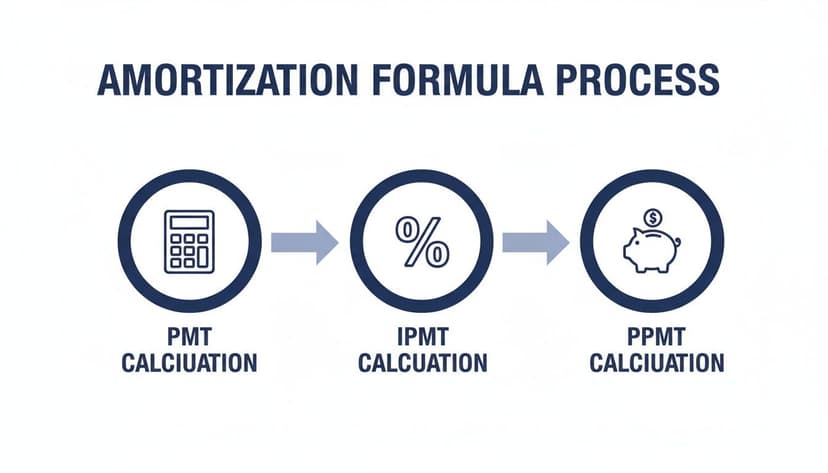
As you can see, the process is logical. First, you calculate the total payment (PMT). Then, for each period, you break that payment down into its interest (IPMT) and principal (PPMT) components.

Now, let's fill these columns with the right formulas. The key here is to use absolute references ($) for your input cells. This is a game-changer because it lets you write the formula once and then drag it down for all other periods, saving a ton of time. An absolute reference like $B$2 tells Excel to always look at cell B2, no matter where you copy the formula.

The secret to an efficient amortization schedule is the dollar sign ($). Using absolute references for your loan inputs prevents formula errors when you drag-fill your table. It’s a small detail that makes a huge difference.

Here’s how to set up the very first row of your schedule, right under your headers (assuming your inputs are in cells B1:B3 and this is row 6):

1. Period: Type the number 1 to start.
2. Beginning Balance: For the first payment, this is your total loan amount. Use a formula like =$B$1.
3. Payment: Use the PMT function: =PMT($B$2/12, $B$3*12, $B$1).
4. Interest: Use the IPMT function for the first period: =IPMT($B$2/12, A6, $B$3*12, $B$1), where A6 is the cell containing "Period 1".
5. Principal: Use the PPMT function: =PPMT($B$2/12, A6, $B$3*12, $B$1). For a deeper dive, learn more about how the PPMT function calculates the principal portion of your payment.
6. Ending Balance: This is a simple calculation: Beginning Balance + Principal. Since the PPMT function returns a negative value, this formula correctly subtracts the principal payment from the balance.

Once the first row is set up, the rest is simple. For the second row, the Beginning Balance will be the Ending Balance from the row above. The other formulas can be dragged down, and they'll adjust perfectly thanks to the mix of absolute and relative references.

See Your Loan Payoff Journey Come to Life

A table of numbers is useful, but visualizing that data in a chart transforms a dense spreadsheet into an at-a-glance snapshot of your financial journey. It’s about turning raw data into a clear picture of progress.

A stacked column chart is perfect for this, as it clearly shows how your payments shift over time—from being mostly interest at the start to almost all principal by the end. Seeing that switch happen visually can be a huge motivator.

From Numbers to Insight

It's often a shock to see just how much of your early payments go to interest. Let’s take a $50,000 business loan at a 7% annual interest rate over 5 years. Your monthly payment is $990.12.

• In the first month, $291.67 of that is just interest.
• By the final month, the interest portion is a mere $9.79.

This visualization is a game-changer for financial planning. Seeing a bar chart where the blue "Interest" portion shrinks month after month is far more impactful than scanning a table. If you're managing a large commitment like a mortgage, getting expert help with your home loan can make all the difference.

Charting Your Progress

Once your amortization table is built, creating a chart is easy. Select the columns with your payment periods, principal payments, and interest payments. Then, go to the Insert tab in Excel and choose a Stacked Column chart.

A stacked column chart is fantastic for pinpointing that 'crossover point'—the exact moment your principal payments finally become larger than your interest payments. It’s a huge milestone on any loan, and seeing it on a graph makes it feel real.

Plotting your loan data provides tangible proof of your progress, which helps you stay motivated on the long road to being debt-free. If you enjoy creating financial visuals, you might also like our guide on how to create a waterfall chart.

Modeling Extra Payments and What-If Scenarios

A basic amortization schedule shows the default path of your loan, but a great one lets you forge a new path. This is where your spreadsheet transforms from a simple tracker into a powerful financial planning tool, giving you a clear picture of how to get out of debt faster.

When you model extra payments, you take direct control over your loan's timeline and, more importantly, its total cost. The setup is simple: add a new column to your schedule labeled "Extra Payment." Here, you can input any extra amount. Then, adjust your "Ending Balance" formula to subtract this extra amount alongside the regular principal payment.

Find Your New Payoff Date with NPER

Once you start making extra payments, the original loan term no longer applies. To find your new freedom date, use Excel’s NPER (Number of Periods) function. It calculates exactly how many payments it will take to pay off a loan.

The syntax is straightforward: NPER(rate, pmt, pv).

• rate: The interest rate for each period (your annual rate divided by 12).
• pmt: Your total payment per period, including your regular payment plus any recurring extra amount.
• pv: The present value, which is your initial loan amount.

Plug in your new, higher monthly payment, and the NPER function will instantly tell you how many months you have left.

Comparing "What-If" Scenarios

This dynamic setup is perfect for running "what-if" analyses. When you're facing big financial decisions, like whether you should renovate or get serious about paying off the mortgage early, this spreadsheet becomes your crystal ball.

You can easily compare different strategies:

• Scenario A: Add an extra $100 to each monthly payment.
• Scenario B: Apply a $5,000 bonus to the loan in the first year.
• Scenario C: Start with an extra $50 now, then increase it to $150 after three years.

Just duplicate your schedule for each scenario to get a side-by-side comparison of interest saved and your new debt-free date.

The true power of an amortization schedule isn't just tracking payments—it's answering the question, "What if?" Every extra dollar you model has a direct, calculable impact, shortening your loan and slashing the interest you'll pay over time.

Let's look at the real-world impact. The table below shows the savings on a typical $200,000, 30-year mortgage at a 6% interest rate by adding a little extra each month.

Impact of Extra Payments on a $200,000 Loan

Extra Monthly Payment	Loan Paid Off In	Total Interest Saved
$50	26 years, 2 months	$30,229
$100	23 years, 1 month	$54,161
$200	18 years, 9 months	$87,949
$500	13 years	$132,160

As you can see, even small, consistent extra payments make a huge difference, shaving years off your loan and keeping tens of thousands of dollars in your pocket.

Let AI Do the Heavy Lifting in Excel

While building an amortization schedule manually is a great way to learn, what if you could achieve the same result in a fraction of the time? AI integrated directly into Excel can make a huge difference.

Instead of hunting for the right cells and remembering the syntax for PMT, PPMT, and IPMT, you can use plain English to tell Excel what you need. The focus shifts from perfecting the formula to simply describing the desired outcome. This approach nearly eliminates small manual errors—a forgotten dollar sign or a wrong cell reference—that can derail your calculations.

From Formula Technician to Financial Strategist

Imagine opening an AI chat panel in your worksheet and typing a simple request.

Example Prompt: "Create an amortization schedule for a $350,000 loan over 30 years at 5.5% annual interest. Include a column for an extra monthly payment of $200 and show the new payoff date."

An AI assistant can interpret that sentence and build the entire table for you in seconds. It sets up the columns, fills them with the correct formulas using absolute and relative references, and even formats the results cleanly. This frees you up to think about the numbers, not the formulas.

This automation lets you move from being a spreadsheet mechanic to a true financial analyst. The real value isn't just in creating the initial table; it's how quickly you can ask follow-up questions and explore scenarios with simple, conversational prompts.

Digging Deeper with Simple Questions

Once the schedule is ready, you can continue the conversation to find more meaningful insights. This is where AI tools prove their worth, giving you instant answers to questions that would normally require building new formulas.

Think about the kinds of follow-up questions you could ask:

• "How much interest will I save with the extra payments? Show me the total."
• "Create a chart showing the principal vs. interest breakdown for the first five years."
• "What would the monthly payment be if the interest rate jumped to 6.25%?"

Each question prompts the AI to run the numbers and show you the answer, turning your static spreadsheet into a dynamic financial modeling tool. If you're curious about the technology, our guide on the AI Excel formula generator explains more. By delegating the repetitive work to AI, you can spend your time interpreting data and making smarter decisions.

Common Questions About Excel Amortization Schedules

As you work with loan amortization in Excel, you’ll inevitably run into a few tricky situations. It’s one thing to build a basic schedule, but another to adapt it to real-world complexities. Here are the most common challenges and how to solve them.

Getting these details right is what separates a decent financial model from a truly reliable one.

How Do I Handle a Variable Interest Rate?

This is a very common question. Standard amortization schedules work perfectly for fixed-rate loans, but what about an adjustable-rate mortgage (ARM)?

The solution is to move away from a single, fixed-rate cell. Instead, add a new column to your schedule titled "Interest Rate." Then, for each payment period (each row), adjust your IPMT, PPMT, and Payment formulas to reference the rate in that specific row.

This small change transforms your static schedule into a dynamic one. You can now manually enter the new rate whenever it changes, and your entire schedule will update automatically to reflect the impact.

What If My Payments Are Not Monthly?

While most loans use a monthly cycle, you might encounter quarterly, bi-weekly, or annual payments. Tweaking your Excel formulas for this is straightforward.

The golden rule is consistency. All your time-based inputs—rate, nper, and per—must use the same time unit.

• Quarterly Payments: Divide your annual interest rate by 4. Multiply the loan term (in years) by 4.
• Bi-weekly Payments: Divide the annual rate by 26. Multiply the loan term by 26.

Seriously, don't forget this. Mismatched units are the single biggest reason people get errors in their loan schedules. If you're calculating a quarterly payment, your interest rate and total periods better be quarterly, too.

Can I Amortize an Operating Lease?

Yes, you can build an Excel schedule for an operating lease, but the setup is different from a standard loan. It’s less about a loan principal and more about a Right-of-Use (ROU) asset and a corresponding lease liability.

You’ll need to add extra columns to track the ROU asset balance and its amortization. The ROU asset is usually amortized on a straight-line basis, meaning the expense is spread evenly over each period of the lease.

While the formulas are more involved than a simple loan, the structured grid of an Excel sheet is still the perfect tool for keeping everything organized and accurate.

---

Ready to stop wrestling with formulas and let AI handle the heavy lifting? Elyx.AI is an AI-powered Excel add-in that builds complete amortization schedules, charts, and financial models from a single plain-English request. Save hours of manual work and get straight to the insights. Try it free for 7 days at https://getelyxai.com.