7 Steps to Master What If Analysis in Excel for Better Decisions

Picture this: you have a crystal ball for your business data. That's pretty much what what-if analysis is in Excel. It's not about predicting the future with 100% accuracy, but about exploring a whole range of possible futures. By tweaking a few numbers in your spreadsheet, you can see the ripple effect on your bottom line almost instantly.

This guide provides practical explanations and real-world examples to help you master what-if analysis, turning you from a passive data viewer into a proactive decision-maker.

1. What Is What If Analysis in Excel?

At its heart, what-if analysis is the process of changing values in your cells to see how those changes impact the results of your formulas. It transforms a static, backward-looking report into a dynamic tool for making smarter decisions, letting you ask all sorts of important questions without messing up your original data.

Think of it as a flight simulator for your business finances. Instead of just staring at last quarter's sales figures, you can use what-if analysis to see what might happen if:

• Your sales jumped by 15% next quarter.
• The cost of your raw materials suddenly increased by 5%.
• You decided to hire two new employees.

This kind of forward-thinking is the backbone of good strategic planning. It helps you get ahead of potential problems, spot hidden opportunities, and make decisions based on a spectrum of possibilities, not just a single, rigid forecast.

The 3 Core Tools for Analysis

Excel comes equipped with a set of built-in features designed specifically for what-if analysis. These tools are your bread and butter for any serious analysis, each built to tackle a different kind of problem. Getting a handle on how they work is key for everything from simple budget tweaks to complex financial models. It's also a must-know skill before you can confidently build a stock tracker spreadsheet to track investments and model future scenarios.

Let's take a quick look at Excel's built-in What-If Analysis tools and what they're best used for.

Core What If Analysis Tools in Excel

Tool Name	What It Does	Best For
Scenario Manager	Creates and saves different groups of input values (scenarios) that you can swap between.	Comparing multiple complex outcomes side-by-side, like a "Best Case," "Worst Case," and "Most Likely" business forecast.
Goal Seek	Works backward from a desired result to find the single input value needed to achieve it.	Situations where you know the outcome you want but need to figure out how to get there (e.g., "How many units do we need to sell to hit $50,000 in profit?").
Data Tables	Shows how changing one or two variables in a formula impacts the final result, all laid out in a grid.	Quickly visualizing the impact of a wide range of inputs on a single output, like how different interest rates and loan terms affect a monthly payment.

Each of these tools offers a unique way to explore your data.

Throughout this guide, we'll dive into each one with some hands-on examples. You can also explore other powerful Excel use cases to see what else is possible.

2. Exploring Excel's 3 Core Analysis Tools

When you want to move past basic calculations and start asking "what if…?", Excel has a powerful set of tools ready to go. You can find them right under the Data tab, and they're built specifically to help you explore different possibilities without the headache of manually changing numbers or creating endless copies of your spreadsheet.

Getting a handle on these three core tools—Goal Seek, Scenario Manager, and Data Tables—is the first real step in turning your static data into a dynamic model for making smarter decisions. Each one is designed for a different kind of question, giving you a complete toolkit for looking at problems from every angle.

This diagram lays it all out, showing how these three distinct features are all part of Excel's "What-If" toolkit, each offering a unique way to explore your data.

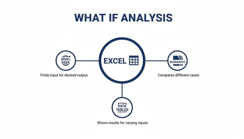
As you can see, each tool branches out from the central idea of what-if analysis, giving you a specific path to test assumptions and see what the future might hold.

2.1. Goal Seek: Your Reverse Calculator

Think of Goal Seek as a simple but brilliant reverse calculator. It’s the most direct of the three tools. You know the answer you want, and you just need Excel to figure out how to get there.

Let's say you're aiming for a $10,000 profit on a new product. Instead of plugging in random numbers for "units sold" until you hit your target, you can just tell Goal Seek:

• Set this cell: The one with your final profit formula.
• To this value: 10000.
• By changing this cell: The one containing the number of units you sell.

Excel does the hard work, instantly calculating the exact number of units you need to sell to hit your $10,000 goal. It’s perfect for those quick, back-of-the-napkin questions where you're just tweaking one variable.

2.2. Scenario Manager: Comparing 3 Different Futures

What happens when you need to change several variables at once? That’s where Scenario Manager shines. It lets you build, save, and compare different sets of input values as complete "scenarios."

Imagine you’re launching a new product. Your team could easily map out a few different realities:

• Best Case: Sales are high, and marketing costs stay low.
• Worst Case: Sales are sluggish, and marketing costs spiral.
• Likely Case: A more realistic middle ground for both sales and costs.

Scenario Manager lets you plug in all the different numbers for each of these versions and then generates a summary report comparing the outcomes. It’s an invaluable tool for planning and risk assessment because it shows you the potential profit or loss for each distinct future. You can even supercharge these models when you learn more about other helpful Excel formulas to build into them.

Key Takeaway: Scenario Manager is your go-to for comparing complex, multi-variable situations. It gives you a structured way to see the big picture when many factors are up in the air, helping you prepare for whatever the market throws at you.

2.3. Data Tables: Running the Numbers on a Grand Scale

Finally, there are Data Tables. This tool is all about seeing how changes in one or two key variables affect your bottom line, all laid out in a single table. It’s a fantastic way to run a quick sensitivity analysis and see just how much your results hinge on certain inputs.

A one-variable data table, for instance, could instantly show you how a monthly loan payment changes as the interest rate climbs from 3% to 7%. A two-variable table can go even further, showing you that same payment change while also factoring in different loan terms (like 15, 20, or 30 years).

You end up with a full matrix of results, giving you a bird's-eye view of how two variables play off each other to impact a critical outcome.

3. How to Use Goal Seek for a Specific Target

Think of Goal Seek as Excel’s reverse engineer. Instead of feeding in numbers and watching a result pop up, you tell Excel the outcome you want—and it works backwards to find the right input. It’s perfect when you know “what” but not the “how.”

Imagine you’re managing a project with a $50,000 cap on spending. You’ve already committed $12,000 in fixed costs, and you expect an external consultant to log 400 hours. Your goal? Pinpoint the highest hourly rate you can pay without busting the budget.

3.1. Setting Up Your Spreadsheet in 4 Steps

Before you dive into Goal Seek, build a simple model that ties everything together. Create cells for fixed expenses, hours, rate, and total cost.

• Fixed Costs (B1): Enter $12,000
• Consultant Hours (B2): Enter 400
• Hourly Rate (B3): Start with a guess, like $50
• Total Cost (B4): Use the formula =B1+(B2*B3). Here's the breakdown:
  • B1 is your fixed cost.
  • (B2*B3) calculates the total consultant cost by multiplying the hours by the rate.
  • The formula adds the fixed cost to the consultant cost for your grand total.

With those entries, your formula in B4 should show $32,000. That gives you a baseline to work from.

Pro Tip: Always lay out your formulas first. Goal Seek relies on a clear link between the result you want and the cell it adjusts.

3.2. Launching and Using Goal Seek in 3 Steps

Now for the fun part—letting Excel do the legwork. In just a few clicks, Goal Seek iterates until your total matches the number you set.

1. Go to the Data tab on the ribbon.
2. In the Forecast group, click What-If Analysis and choose Goal Seek.
3. Fill in the dialog:
   • Set cell: B4 (your total cost formula)
   • To value: 50000
   • By changing cell: B3 (hourly rate)

Click OK, and Excel will adjust B3 until B4 hits exactly $50,000. You’ll discover the consultant’s top billable rate is $95—all without a manual guess-and-check marathon.

4. How to Manage Scenarios with Scenario Manager

When you're juggling a handful of different variables to see how things might play out, Excel's Scenario Manager is your best friend. It’s perfect for more complex planning, like trying to forecast the success of a new marketing campaign where a few key factors could swing either way.

Let’s walk through building a model for a digital ad campaign to see this tool in action.

For our campaign, profitability really boils down to three key variables: the total ad spend, the click-through rate (CTR), and the conversion rate from those clicks. We’ll use Scenario Manager to create three distinct versions of the future—a best case, worst case, and a realistic middle ground—to compare them all side-by-side.

4.1. Setting Up the 3-Part Campaign Model

First thing's first: you need to structure your spreadsheet. You’ll need cells for your inputs (the variables you'll be changing) and cells for your outputs (the results you want to keep an eye on).

A simple setup might look like this:

• Ad Spend (B1): $10,000
• Click-Through Rate (B2): 2.0%
• Conversion Rate (B3): 5.0%

Next, you'll need some formulas to calculate the results based on those inputs. For example:

• Total Clicks (B5): Use the formula =(B1/0.50)*B2. This formula calculates your total clicks based on ad spend and a fixed Cost-Per-Click (CPC) of $0.50. (B1/0.50) determines how many impressions or actions your budget buys, and multiplying by the CTR (B2) gives you the number of clicks.
• Total Conversions (B6): Use the formula =B5*B3. This is a straightforward calculation: Total Clicks * Conversion Rate equals the number of successful conversions.
• Revenue (B7): Use the formula =B6*25. This multiplies your total conversions by the value of each conversion ($25) to find total revenue.
• Profit (B8): Use the formula =B7-B1. This calculates your net profit by subtracting your initial ad spend from the total revenue generated.

This initial setup is our "Realistic" or baseline scenario. It's our starting point.

4.2. Defining Your 3 Scenarios

With the basic model built, it's time to add your different scenarios. You'll find the tool by navigating to Data > What-If Analysis > Scenario Manager and clicking "Add" to create each one.

1. Realistic Scenario: This is your baseline. Name it "Realistic," and for the "Changing cells," select B1, B2, and B3. The current values are already what you need, so you can just save it.
2. Optimistic Scenario: Now, add a new scenario and call it "Optimistic." The changing cells (B1:B3) will be the same. In the next window, plug in your best-case values: maybe an Ad Spend of $12,000, a CTR of 3.0%, and a rosy Conversion Rate of 7.0%.
3. Pessimistic Scenario: Lastly, create a "Pessimistic" scenario. Here, you might dial back the Ad Spend to $8,000, with a CTR of just 1.5% and a Conversion Rate of only 3.5%.

Important Note: While Scenario Manager is a powerful tool for comparing different outcomes, setting it all up is still a very manual process. Creating and managing multiple models this way is a common headache for many teams.

This reliance on manual work is surprisingly common. A 2023 Forrester survey found that 82% of organizations still depend on manual processes built around Excel, which creates some major bottlenecks. Professionals often sink over three hours a week on these kinds of tasks, which really underscores the need for better automation. To see how AI can take on this kind of work, you can learn more about AI automation in Excel.

4.3. Generating a Scenario Summary Report in 2 Clicks

Once all your scenarios are defined and saved, just click "Summary" in the Scenario Manager window. Excel will ask which cells contain your results—in our case, that would be B7 for Revenue and B8 for Profit. Select those and click OK.

Instantly, Excel generates a brand-new worksheet with a perfectly formatted summary report. This table neatly lays out the inputs and outcomes for your Realistic, Optimistic, and Pessimistic scenarios, giving the marketing team a crystal-clear, at-a-glance view of the potential ROI. This lets them build a much more resilient strategy, because they're walking in fully aware of the best, worst, and most likely financial outcomes of their campaign.

5. How to Run Sensitivity Analysis with 2 Data Tables

While Scenario Manager is great for comparing a few specific, hand-picked outcomes, Data Tables are the tool you need when you want to see how one or two changing numbers affect your entire model. Think of it as a stress test. You can see exactly how sensitive your final result is to a continuous range of inputs, which is incredibly useful for financial modeling and risk assessment.

Let's walk through how to build both a one-variable and a two-variable table. We'll stick with a classic example: figuring out how different interest rates and loan terms change a monthly loan payment.

5.1. Creating a One-Variable Data Table

Imagine you’re considering a $300,000 loan over 30 years. You want to see how your monthly payment would change if the interest rate isn't what you expect.

First, build a simple model in your spreadsheet:

• Loan Amount (B1): 300000
• Term in Years (B2): 30
• Interest Rate (B3): 5.0% (this is the number we'll be changing)

Next, you need a formula to calculate the payment. In cell B5, use Excel's PMT function: =PMT(B3/12, B2*12, -B1). Here’s a detailed explanation:

• rate (B3/12): The interest rate for the period. Since B3 is an annual rate, we divide by 12 for a monthly rate.
• nper (B2*12): The total number of payments. We multiply the term in years by 12.
• pv (-B1): The present value, or the total loan amount. It's entered as a negative number because it's cash you receive (an inflow).

Now, it's time to set up the table itself. In a single column (let's say D2 through D8), list out the different interest rates you want to test—maybe 4.0%, 4.5%, 5.0%, and so on. In the cell just above and to the right of your list (E1), you need to link back to your original calculation. Simply type =B5 into cell E1.

Here’s how to make the magic happen:

1. Select the whole range, including your list of rates and the linked formula cell (in our case, D1:E8).
2. Head to the Data tab, click What-If Analysis, and choose Data Table.
3. A small dialog box will pop up. Since your changing values (the interest rates) are in a column, you’ll use the Column input cell field.
4. Click into that field and select your original interest rate cell, which is B3.
5. Click OK. Excel will instantly fill in the table, calculating the monthly payment for every single rate you listed.

5.2. Building a Two-Variable Data Table

Ready to get more sophisticated? A two-variable table takes this what if analysis to the next level by letting you see how two inputs—like interest rate and loan term—interact.

Your initial model stays the same, but the table layout needs to change. Keep your interest rates running down the column (D2:D8). Now, list your second set of variables, the loan terms (e.g., 15, 20, 25, 30 years), across the top row (E1:H1).

The top-left corner cell (D1), where the row and column meet, is crucial. This cell must point back to your original payment formula. So, in cell D1, enter =B5.

To generate the full matrix:

1. Select the entire table range, from the corner cell to the last data point (D1:H8).
2. Go back to Data > What-If Analysis > Data Table.
3. For the Row input cell, select the cell from your original model that holds the loan term (B2).
4. For the Column input cell, select the cell that holds the interest rate (B3).
5. Click OK.

Instantly, you have a complete grid showing how the monthly payment changes with every possible combination of rate and term. Trying to build this matrix by hand would be tedious and prone to error, but Data Tables automate the whole process.

This kind of automation is a huge deal in the business world. In fact, the market for workflow automation hit $20.3 billion in 2023 and is only expected to grow.

Tools like Data Tables give you a taste of what’s possible with automated analysis. For even more powerful options, you can see how artificial intelligence is enabling deeper AI data analysis in spreadsheets.

6. How to Automate Analysis with AI in Excel

While Excel’s built-in what-if tools are incredibly useful, let's be honest—they can take a lot of manual work to set up. The biggest headache with what-if analysis isn't the concept, it's the time suck. Building the models, tweaking the formulas, and defining every single scenario can eat up hours. This is exactly where new AI tools are stepping in to change the game.

Tools like the autonomous AI agent ElyxAI are designed to get rid of that friction. Instead of clicking through menus and filling out dialog boxes, you can just ask for what you need in plain English.

Think about it. You could simply type: "Show me how a 10% and 20% increase in shipping costs affects my profit margin for Product X."

The AI understands your question, runs the numbers in the background, and gives you the answer right in your spreadsheet. This completely changes your workflow. You stop wrestling with the how and get to focus on the what—using the results to make smarter decisions.

The Power of Conversational Commands

This shift to conversational AI is more than just a neat trick; it's a major trend. The market for automation solutions is expected to grow from $163.54 billion in 2025 to a staggering $262.572 billion by 2033. For anyone who lives in spreadsheets, AI completely flips the script on manual tasks, with many people saving over three hours a week.

ElyxAI is a great example of this new wave, especially with its privacy-first design. It can handle complex requests without your data ever leaving your computer, which is a huge step up from older, cloud-based methods.

Key Insight: AI agents turn what-if analysis from a complicated, multi-step process into a simple conversation. This opens up sophisticated analysis to everyone, not just Excel experts.

Instead of spending an afternoon building a model, you can get answers in seconds. This speed lets you explore more possibilities and be more creative with your scenarios, which ultimately leads to stronger, data-backed strategies.

By letting an AI assistant handle the technical heavy lifting, you free up your brainpower for the important stuff: critical thinking and strategic planning. You can see the full range of possibilities by learning more about what an Excel AI assistant can do.

7. 3 Common Questions About What-If Analysis

Let's tackle a few common questions that come up when people start exploring what-if analysis in Excel.

7.1. Can a What-If Analysis Be Wrong?

Absolutely. The old saying, "garbage in, garbage out," is especially true here. The results of your analysis are only as reliable as the assumptions and data you start with.

Think about it this way: if you build a "best-case scenario" based on a completely unrealistic sales forecast, the final numbers will look fantastic, but they won't mean anything. That’s why it’s so important to sanity-check your assumptions before you start plugging them into a model and making decisions based on the output.

7.2. What's the Difference Between Sensitivity Analysis and What-If Analysis?

This is a great question, and it's easy to get them mixed up. The simplest way to remember it is that sensitivity analysis is just one type of what-if analysis.

"What-if analysis" is the big-picture term for changing any input variable to see how it affects the outcome. Sensitivity analysis is more focused. It's specifically about isolating one key variable (like an interest rate or a material cost) and seeing how sensitive a specific result (like your total profit) is to changes in that single input. In Excel, this is exactly what Data Tables are designed to do.

7.3. Why Bring AI Into This?

Using AI is all about speed and simplicity. Instead of spending your time manually setting up the models, creating data tables, and running different scenarios, you can just ask a question.

AI tools handle the tedious setup for you. You can describe the analysis you want in plain English, and the AI builds the model and delivers the results, letting you focus on the insights, not the mechanics.

---

Ready to stop building manual models and start getting instant answers? Elyx AI acts as your autonomous Excel agent, turning complex requests into finished analyses in seconds. See how much time you can save.