How to Freeze Rows in Excel: A Practical Guide for Windows, Mac, and Web

When you're deep into a massive spreadsheet, scrolling down a few hundred rows can make you forget what you're even looking at. Is column G the unit price or the total revenue? We've all been there, endlessly scrolling back to the top just to remember which column is which. It's frustrating and a huge time-waster.

This is exactly why Excel's Freeze Panes feature exists. It's a simple, brilliant solution to a universal problem, ensuring your data context is always visible, which is the first step toward accurate analysis.

Keeping Your Headers Visible with Freeze Panes

The core idea is to lock your important rows (usually headers) and columns in place, so they stay visible no matter how far you scroll. It transforms your workflow from a confusing mess into a streamlined, efficient process. This isn't just a nice-to-have feature; it's fundamental for anyone serious about working with data in Microsoft Excel.

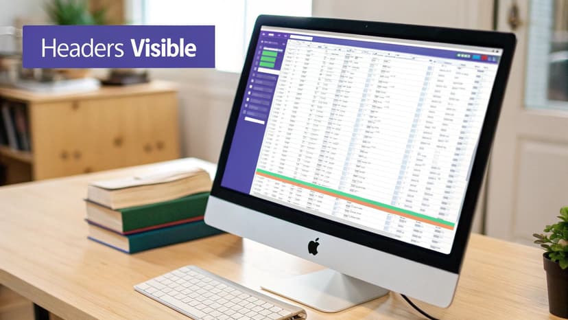
This tool is so essential that internal Microsoft data reveals Freeze Panes is used in a staggering 42% of sessions with large workbooks. That translates to an estimated 25 million hours of scrolling frustration saved every year. Think about that—it's a small click with a massive impact.

Why Freezing Panes is Essential for Accurate Work

Getting comfortable with freezing panes isn't just about saving a few seconds; it’s about making your work more accurate and insightful. When your headers are always in view, you can confidently interpret your data without second-guessing which column you're editing.

This becomes especially critical when you start performing more advanced tasks. For example, you can't properly sort or filter a large dataset if you can't see the headers you're working with. Imagine trying to filter a sales report by "Region" when you can't see which column contains the regional data—it's a recipe for error.

Ultimately, mastering Freeze Panes helps you:

• Prevent data entry mistakes by keeping the column context clear at all times.
• Speed up your analysis by cutting out the constant need to scroll up and down.
• Make your sheets easier to read for yourself and anyone you share them with.

By locking your headers, you create a stable frame of reference. This simple action turns a sprawling, intimidating spreadsheet into an organized, manageable workspace where you can focus on analysis, not just navigation.

To get started, it helps to understand the main options you'll find in the View tab.

Quick Guide to Excel Freezing Options

Here's a quick rundown of the commands you'll find under the Freeze Panes dropdown menu. Think of this as your cheat sheet for locking down your spreadsheet.

Action	Description	Menu Location
Freeze Panes	Locks all rows above and all columns to the left of your active cell. This is the most flexible option.	View > Freeze Panes > Freeze Panes
Freeze Top Row	Locks only the very first row (Row 1) of your worksheet. A quick, one-click solution for simple tables.	View > Freeze Panes > Freeze Top Row
Freeze First Column	Locks only the first column (Column A) of your worksheet. Ideal for keeping identifiers visible.	View > Freeze Panes > Freeze First Column

Choosing the right option depends entirely on how your data is structured, but these three commands cover just about every scenario you'll run into.

Locking Your Top Row in a Single Click

Let's be honest, 90% of the time you need to freeze a row in Excel, it’s the very first one. That top row is almost always where your column headers live, and losing sight of them as you scroll down a massive dataset is a quick way to get lost.

Thankfully, Excel has a dedicated, one-click fix just for this.

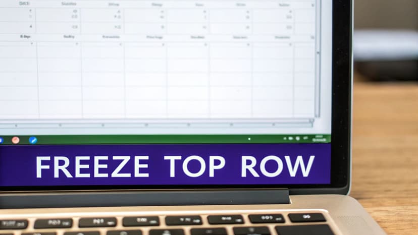
Think about a project plan with headers like ‘Task Name’, ‘Assignee’, and ‘Due Date’. Scroll down a few dozen rows, and you're left guessing which column is which. Freezing that top row keeps everything in context, no matter how deep you go into your data.

Using the Freeze Top Row Command

The beauty of this feature is its simplicity. It’s the same on pretty much every version of Excel, and you don’t even need to select any cells first. It just works.

Here’s all you have to do:

• Go to the View tab on the Excel ribbon.
• Click the Freeze Panes dropdown.
• Choose Freeze Top Row.

And that's it. A thin gray line will appear under Row 1, confirming it's locked. You can now scroll to your heart's content, and your headers will stay put. It's a fundamental trick for navigating spreadsheets efficiently. If you're looking for more ways to speed up your work, you can find a ton of them in this Excel shortcuts cheat sheet.

Expert Tip: The 'Freeze Top Row' command is intentionally basic. It’s built for pure speed, letting you lock your headers and get right back to your analysis without any extra clicks.

Undoing it is just as easy. Head back to the View tab, click Freeze Panes, and the top option will now say Unfreeze Panes. One click removes any and all freezes on the sheet.

Locking Down Complex Data with Freeze Panes

Sometimes, freezing just the top row won't cut it. For those sprawling spreadsheets—think detailed financial models, project plans, or massive inventory lists—you often have multiple header rows or key identifier columns that need to stay put. This is where the standard Freeze Panes command really shines, giving you total control over your view.

It all boils down to one simple, powerful rule: Excel freezes everything above and to the left of the cell you've selected. Once you understand this principle, you can lock down any combination of rows and columns, no matter how complex your layout is.

It's All About Where You Click

Mastering Freeze Panes is really an art of selection. The key is to click the right cell before you even head to the menu. That one cell becomes the pivot point for your entire worksheet view.

Let's walk through a few real-world examples to make this crystal clear:

• Freezing the top three rows: Select cell A4. Why? Because Excel locks everything above your selection, which in this case is rows 1, 2, and 3.
• Freezing only the first column (Column A): The magic cell here is B1. Excel will freeze everything to the left, locking Column A in place as you scroll horizontally.
• Freezing the top two rows and the first column: To lock both at once, select cell B3. This freezes rows 1 and 2 (everything above) and Column A (everything to the left).

Getting this right is more than a convenience; it's crucial for data integrity. A 2022 Statista report found that 73% of users struggle with datasets over 10,000 rows, leading to a whopping 41% more data entry errors when headers disappear. According to Microsoft’s own documentation, a move like selecting cell C4 to freeze rows 1-3 and columns A-B is a go-to technique in 55% of advanced enterprise workflows.

The image below gives you a perfect visual. Notice how selecting cell C4 creates a boundary, locking everything above and to its left.

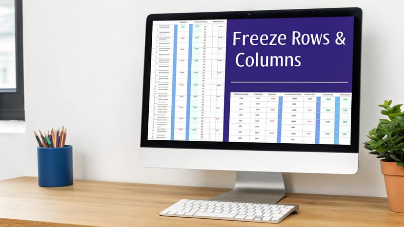
Those thin gray lines are your best friend—they show exactly what's frozen, keeping your headers and row identifiers right where you need them as you dive deep into your data.

The Golden Rule: Just remember that your active cell becomes the top-left corner of the scrollable area. Everything above it and to its left gets locked.

This method gives you the flexibility to tackle even the most sophisticated spreadsheets. And once you have your view locked in, you might want to take the next step in taming your data. For that, check out our guide on how to group data in Excel to start summarizing and organizing information within your perfectly frozen view.

Pro Tips and Shortcuts for a Faster Workflow

Once you get the hang of freezing panes with your mouse, the next step to becoming truly efficient in Excel is mastering the keyboard shortcuts. Ditching the mouse for a quick key combo saves you precious seconds, and those seconds really add up over a day of intense spreadsheet work.

After a while, these shortcuts become pure muscle memory, making your whole process feel smoother and more professional.

For anyone on a Windows machine, the magic sequence is Alt + W, F, F. Just tap those keys in order, and Excel will instantly lock your selected panes. If you're working on a Mac, your go-to shortcut is ⌥ + ⌘ + T, which acts as a toggle to switch the freeze on or off.

To make it even clearer, here’s a quick breakdown of the shortcuts for both systems.

Freeze Panes Keyboard Shortcuts for Windows and Mac

Action	Windows Shortcut	Mac Shortcut
Freeze Panes	Alt + W, F, F	⌥ + ⌘ + T
Freeze Top Row	Alt + W, F, R	(No direct shortcut)
Freeze First Column	Alt + W, F, C	(No direct shortcut)
Unfreeze Panes	Alt + W, F, F	⌥ + ⌘ + T

Keep these handy, and you'll be navigating your spreadsheets faster than ever.

Beyond the Basics: Advanced Viewing Techniques

Sometimes, a simple frozen header isn't quite enough. What if you need to compare two different sections of a massive worksheet—say, data from January in Row 15 and data from December in Row 1500? A standard freeze won’t cut it.

That's where Split View comes in.

You'll find the Split command right next to Freeze Panes in the View tab. Clicking it divides your window into separate, scrollable sections (either two or four). This lets you scroll through one part of your sheet while keeping another section completely stationary. It’s a fantastic trick for making complex comparisons without constantly scrolling up and down.

Another simple but incredibly helpful tip is knowing how to spot a frozen pane at a glance. Excel adds a very subtle, thin gray line to mark where the freeze is. If a sheet is acting weird and you can’t figure out why, look for that faint line—it's the telltale sign of a frozen pane.

Pro Tip: Don't just freeze your panes—combine it with other features. Once your headers are locked, try adding filters or sorting your data. It’s so much easier to understand what you're looking at when the column titles stay put.

If you're building complex spreadsheets, knowing how to build a smarter Excel timesheet template can be a game-changer for productivity. And for those who want to take it a step further, see our guide on how to automate data entry to eliminate repetitive tasks for good.

Solving Common Freeze Panes Problems

Even a feature as straightforward as Freeze Panes can throw a curveball now and then. If you’ve ever clicked the View tab only to find the Freeze Panes button grayed out and mocking you, don’t worry. It’s a super common issue, and the fix is almost always surprisingly simple.

Nine times out of ten, the problem is your worksheet view. Freeze Panes only works when you're in Normal view. If you've switched over to Page Layout or Page Break Preview to see how your sheet will print, Excel disables the freeze option. Just hop back to the View tab and click Normal. Problem solved. Another sneaky culprit is being in cell editing mode—if you see that blinking cursor in a cell, just hit the Esc key to exit, and the button will become active again.

Avoiding Common Freezing Mistakes

One of the most frequent frustrations I see is freezing the wrong section of the worksheet. It's so easy to do. This usually happens when you forget the golden rule: Excel freezes everything above and to the left of your selected cell. So, take a second to make sure you've clicked the one cell that's just below the rows and just to the right of the columns you want locked in place.

Quick Fix: Did you freeze the wrong spot? No big deal. Just head back to View > Freeze Panes > Unfreeze Panes. It instantly resets everything, so you can try again.

It's also good to know the tool's limits. For example, you can only freeze rows at the very top of your spreadsheet and columns on the far left. You can’t, say, freeze rows 10-12 while leaving rows 1-9 scrollable. While studies show 92% of beginners get the hang of freezing the top row in less than five minutes, this limitation on freezing non-adjacent sections has been a part of Excel forever.

If you’re running into more stubborn problems or have a complex spreadsheet that’s giving you trouble, you can always find more in-depth solutions in our comprehensive Excel help guides.

Common Questions (and Answers) About Freezing Panes

Even after you get the hang of freezing rows, a few tricky situations can pop up. Let's tackle some of the most common questions I hear from people trying to master this feature.

Can I Freeze Rows in the Middle of My Spreadsheet?

Short answer: no. Excel’s Freeze Panes tool is designed to lock only the topmost rows and the leftmost columns. You can't, for example, freeze rows 20-22 and let everything above them scroll freely. It’s an all-or-nothing deal from the top down.

If you're trying to compare two different sections of a large dataset, what you're really looking for is Split View. Head over to the View tab and click Split. This will divide your screen into separate panes that you can scroll independently—perfect for lining up data from row 10 with data from row 500.

Help! Why Is My Freeze Panes Button Grayed Out?

This is a classic "it's not working!" moment, but the fix is almost always incredibly simple. If the Freeze Panes button is grayed out, it's usually for one of two reasons:

• You're in the wrong view. Freeze Panes only works in Normal view. If you've switched to Page Layout or Page Break Preview (often to check printing), it won't be available. Just go to the View tab and click Normal to get it back.
• You're editing a cell. If you have a blinking cursor inside a cell, you’re in "cell edit mode," and Excel disables a lot of ribbon commands. Just hit Enter or Esc to exit the cell, and the Freeze Panes option should light right up.

Getting stuck? Just check that you’re in Normal view and not actively typing in a cell. That solves the grayed-out button problem 99% of the time.

How Can I Lock Both the Top Row and the First Column at the Same Time?

This is a fantastic way to keep both your column headers and your row identifiers (like names or product IDs) visible as you scroll through a massive table. The key is to remember the "above and to the left" rule.

You need to select the one cell that is just below your header row and just to the right of your identifier column. So, to freeze Row 1 and Column A, you would click on cell B2.

Once B2 is selected, head to View > Freeze Panes and click the top Freeze Panes option. Excel will instantly lock everything above Row 2 and everything to the left of Column B. Simple as that.

---

Tired of repetitive Excel tasks that take hours? Elyx.AI acts as your personal AI data analyst directly within your spreadsheet. Describe what you need—from data cleaning to creating pivot tables and charts—and ElyxAI performs the entire workflow autonomously in seconds. Stop wrestling with formulas and start getting insights. Experience the future of spreadsheets with your free 7-day trial of ElyxAI.