A Practical Guide on How to Concatenate in Excel

If you need to quickly combine text in Excel, the simplest way is to use the ampersand (&). A formula like =A2&" "&B2 is all it takes to join the text from cell A2, add a space, and then add the text from cell B2. It's an essential technique for fast and simple text merging.

Your Guide to Combining Text in Excel

Ever find yourself with columns of data that belong together? Think first names and last names, or separate parts of an address. Knowing how to concatenate in Excel is one of those fundamental skills that turns fragmented data into something useful, saving you a ton of manual copy-and-pasting. The goal is simple: merge text from multiple cells into one. Luckily, Excel gives us several ways to get this done, from basic symbols to powerful, modern functions.

This guide will provide practical explanations and real-world examples to solve this concrete problem. We'll start with the most direct methods—the ones you can use right now—and then build up to more advanced techniques for tackling trickier data-joining challenges, including how AI can streamline the process.

The Classic Concatenation Methods

For years, Excel users have relied on two main tools for combining text: the ampersand (&) operator and the CONCATENATE function. Of the two, the ampersand is often preferred for its sheer simplicity and speed.

Let's say you have a list of products in one column and their model numbers in another. To create a clean product ID, you could just type =B2&"-"&C2. This formula instantly joins the product name from B2, a hyphen, and the model number from C2.

The ampersand method is highly visual; you can see exactly how your new text string is being built in the formula bar. It's incredibly handy for quick, one-off jobs.

Actionable Tip: Remember, Excel won't add spaces or punctuation for you. You have to explicitly tell it to. Always include your delimiters—like a space (" "), a comma and space (", "), or a hyphen ("-")—inside double quotes. This is the key to making your final text readable and solving the common issue of jumbled text.

Understanding the CONCATENATE Function

The other classic tool is the CONCATENATE function. Writing =CONCATENATE(A2, " ", B2) accomplishes the exact same thing as the ampersand, just with a more formal function structure.

For a long time, this was the standard function for combining text. It could handle up to 255 different text arguments and create a string up to 8,192 characters long. However, starting with Excel 2016, Microsoft began phasing it out in favor of the newer, more efficient CONCAT function. You can read more about the history of Excel's text functions if you're curious.

While CONCATENATE still works for backward compatibility, it's a good practice to start using its modern replacements. They offer better functionality and align with current Excel standards.

Using CONCAT and TEXTJOIN Like a Pro

While the ampersand and the old CONCATENATE function work, modern Excel offers much smarter tools for the job. Let’s dive into two functions that have largely made the old ways obsolete: CONCAT and the incredibly powerful TEXTJOIN.

These aren't just slight improvements; they fundamentally change how you can tackle text-joining tasks, making your formulas shorter, cleaner, and far more capable. This is an upgrade in efficiency, much like moving from a manual screwdriver to a power drill.

The CONCAT Function: A Welcome Upgrade

CONCAT is the direct replacement for CONCATENATE. On the surface, it seems almost identical, but it has one massive advantage that makes all the difference: it accepts cell ranges.

With the legacy CONCATENATE function, if you needed to join text from cells A1 through C1, you had to type out each cell reference individually: =CONCATENATE(A1, B1, C1). This becomes tedious if you have many cells to join.

CONCAT simplifies this beautifully. You can just write =CONCAT(A1:C1) to get the exact same result. This ability to use a range makes formulas much easier to write and maintain, especially when you're working with long rows of data.

Key Takeaway: The single biggest reason to switch to CONCAT is its support for ranges. When you need to join a series of adjacent cells, =CONCAT(A1:E1) is far more efficient than listing every single cell with an ampersand or the clumsy CONCATENATE function.

Master Lists with the TEXTJOIN Function

TEXTJOIN is a game-changer for anyone who has ever tried to build a clean, separated list from various cells. It solves two of the biggest concatenation headaches with one simple, elegant formula.

The syntax for TEXTJOIN is: =TEXTJOIN(delimiter, ignore_empty, text1, [text2], ...)

Let's break down its powerful arguments:

• Delimiter: This is the character you want to place between each item. It could be a comma and a space (", "), just a space (" "), a hyphen ("-"), or any other separator.
• Ignore_empty: This is a simple TRUE or FALSE. If you set it to TRUE, TEXTJOIN will automatically skip any blank cells in your selection. This is a brilliant feature that prevents ugly double delimiters (like ", ,") from cluttering your final text.
• Text1, [text2], …: This is the text you want to join. Like CONCAT, this can be individual cells or, more usefully, an entire cell range.

Real-World Example: Let’s say you have an address spread across several columns: "123 Main St" in A2, a blank cell in B2 (for an apartment number), "Anytown" in C2, and "CA" in D2.

Using TEXTJOIN, you can create a perfect, comma-separated address with one quick formula: =TEXTJOIN(", ", TRUE, A2:D2).

The result is: "123 Main St, Anytown, CA".

Notice how it automatically inserted the ", " between each piece of text and, crucially, completely ignored the empty cell in B2. Achieving this result with older methods would have required a much more complicated and error-prone formula. Even with powerful functions, formulas can sometimes go wrong. If you get stuck, a good guide on Excel formula troubleshooting can be a real lifesaver.

Handling Formatting and Line Breaks

One of the first real headaches users encounter when combining text in Excel is format loss. You might have a perfectly formatted date, say "Dec 25, 2024," and you try to join it with some text. The result is often something bizarre like "Shipment arriving on 45650".

This happens because Excel stores dates, times, currencies, and percentages as numbers internally. The formatting you see is just a visual layer. When you concatenate, Excel grabs that raw, underlying number, completely ignoring the visible formatting. Thankfully, a specific function is built to solve exactly this problem.

Keep Your Numbers Looking Right with the TEXT Function

The TEXT function is your go-to tool for preserving number formats within a concatenation formula. It converts a number into a text string while applying the specific formatting you define. It essentially tells Excel, "Take this number, but make sure it looks like a date or a dollar amount before you join it."

The syntax is straightforward: =TEXT(value, "format_code").

You nest this function right inside your main concatenation formula. Let's look at a practical example. Imagine you have a product price of $49.99 in cell B2 and a sales date of 12/1/2024 in cell C2.

• For Currencies: Instead of = "Price: " & B2, you'd write = "Price: " & TEXT(B2, "$#,##0.00"). Now your output is the clean "Price: $49.99".
• For Dates: Rather than = "Sale Date: " & C2, the proper formula is = "Sale Date: " & TEXT(C2, "mmm d, yyyy"). This gives you the readable "Sale Date: Dec 1, 2024".

The format codes are incredibly flexible, allowing you to achieve almost any look you want, from percentages ("0.0%") to various date styles ("dd-mm-yy").

How to Add a Line Break in an Excel Cell

Sometimes you need to stack information vertically inside a single cell, such as when creating a mailing address. Simply pressing Enter in the formula bar won't work. The solution is to use a special character that Excel interprets as a line break.

That character is generated by the CHAR(10) function. In ASCII character codes, the number 10 represents a line feed.

Let's say you have a street address in A2 ("123 Maple Lane"), a city in B2 ("Oakville"), and a state/zip in C2 ("FL 33101"). To combine these into a properly stacked address, your formula would be:

=A2 & CHAR(10) & B2 & CHAR(10) & C2

Don't Forget This Step: After you enter the formula, the result will likely appear as a single long line of text. To make the line breaks visible, you must enable Wrap Text. Select the cell (or the whole column), go to the Home tab, and click the Wrap Text button in the Alignment section. Your text will now be neatly stacked, making your data presentation much more professional.

Advanced Merging with Power Query

When you're dealing with hundreds of rows, worksheet formulas are effective. But what happens when that number balloons to thousands, or even millions? Your spreadsheet's performance can degrade. For these larger jobs or repetitive tasks, Excel has a much more powerful tool: Power Query.

Instead of typing a formula into a cell and dragging it down, Power Query lets you build an automated, repeatable process for data transformation. Think of it as creating a recipe that Excel can follow every single time new data comes in. It performs these operations without altering your original source tables, keeping your raw data safe and your workflow clean.

Your First Steps with Power Query Merging

Getting started with Power Query is quite straightforward. First, you need to load your data into the Power Query Editor. Select your data range or table, navigate to the Data tab, and click on From Table/Range.

Once inside the Power Query Editor, the transformation begins:

• Hold down the Ctrl key and select the columns you want to combine. Ensure you click on them in the exact order you want them to appear in the merged column.
• Next, go to the Add Column tab in the ribbon.
• From there, click the Merge Columns button.

A dialog box will appear, allowing you to choose a separator—like a space, a comma, or a custom character—and name your new merged column. Once you click OK, Power Query applies the merge operation to your entire dataset instantly.

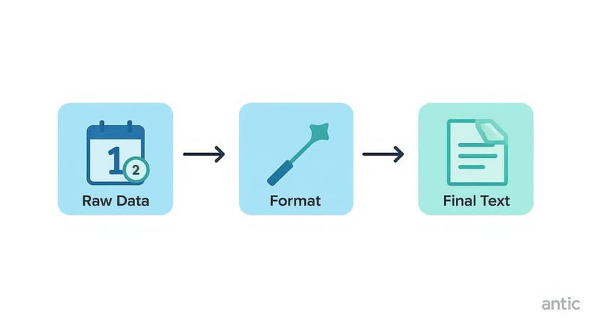
This diagram illustrates how Power Query transforms separate pieces of raw data through a defined process into a clean, final text string.

This workflow highlights the core value of Power Query: creating a systematic process for turning messy inputs into a polished, usable output.

The Power of a Refreshable Query

The true strength of using Power Query lies in its "set it and forget it" nature. After setting up your merge steps, you just click Close & Load. This sends your transformed data back into a new Excel worksheet.

The key benefit: your query is now a live connection. If your original source data changes—new rows are added, or text is updated—you don't need to rebuild anything. Simply right-click your new table and hit Refresh, and Power Query instantly re-runs all your steps, updating the merged column automatically.

This level of automation is a significant leap forward from manually managing formulas. Power Query is not only a powerful tool within Excel but also a core component of comprehensive Business Intelligence software solutions like Power BI, where it handles even larger-scale data analytics.

Automating Concatenation with AI Tools

We’ve walked through effective ways to join text in Excel, from basic formulas to the robust capabilities of Power Query. They all solve the problem. But what if you could skip writing formulas altogether?

This is where artificial intelligence is changing the game inside Excel. Instead of you needing to know Excel's specific syntax, AI tools can understand your natural language instructions.

From Instruction to Instant Formula

AI assistants built for Excel, like Elyx.AI, allow you to simply describe what you want to achieve in plain English. There’s no syntax to remember and no functions to look up, which dramatically speeds up the process of solving your problem.

For example, with first names in column A and last names in column B, you could stop and think, "Okay, I need to select A2, add an ampersand, then a quote with a space, another quote, another ampersand, and then B2."

Or, you could just tell the AI: "Combine the first name in column A and the last name in column B, separated by a space."

The AI assistant understands the request and instantly generates the correct formula, =A2&" "&B2, ready for you to use. It’s not just faster; it’s more accurate. It sidesteps the tiny, frustrating syntax errors like a forgotten quote or a missing & that can bring your work to a halt. You can see more on how an AI Excel formula generator can solve these common headaches.

This shifts your role from being a formula writer to a project manager. You state the goal, and the AI builds the solution.

The real value of using AI in Excel is how it translates your intent directly into a working formula. It closes the frustrating gap between knowing your goal and knowing the exact syntax to make Excel execute it. Suddenly, complex tasks become accessible to everyone.

The Broader Impact of AI Automation

This kind of natural language automation is not limited to spreadsheets. The concept of commanding software with simple instructions is making office work more efficient across various applications. To understand the bigger picture, it's worth exploring how AI tools can automate tasks across different applications, from data analysis to building presentations.

By integrating an AI tool into your Excel workflow, you can:

• Save Significant Time: Repetitive combining tasks that used to take up valuable time can now be handled in seconds.
• Reduce Frustration: Eliminate the trial-and-error process with tricky TEXTJOIN formulas or nested TEXT functions.
• Increase Productivity: Tackle complex merges and formatting jobs without needing to be a formula expert.

Ultimately, using AI for tasks like concatenation is about working smarter. It allows you to spend more of your cognitive energy on analyzing the data, not just on the manual effort of preparing it.

Got Questions? I've Got Answers

Once you get the hang of concatenating in Excel, you'll inevitably run into a few tricky situations. Here are some of the most common questions that arise and how to handle them effectively.

Why Did My Date Turn Into a Weird Number?

This is the classic "date-to-serial-number" problem. You try to join "Report Date: " with a cell containing "1/1/2024," and you get something like "Report Date: 45291." It's one of the most common frustrations for anyone new to concatenation.

This happens because Excel stores dates as serial numbers internally. To fix it, you must explicitly tell Excel to format the date as text before joining it. The TEXT function is your solution.

Instead of ...& A1, wrap it like this: ="Report Date: " & TEXT(A1, "mm/dd/yyyy"). This forces the date into the format you want before it gets combined.

How Can I Clean Up All These Extra Spaces?

You import some data and notice the concatenated names look off, like "John  Smith". This is usually because the original cells have stray leading or trailing spaces. The TRIM function is designed specifically for this scenario; it removes any extra spaces from the beginning or end of a text string.

The trick is to wrap each cell reference with TRIM inside your concatenation formula.

For example, a formula like =TRIM(A2) & " " & TRIM(B2) cleans up both the first and last name cells before joining them, resulting in a perfectly clean "John Smith."

What's the Best Way to Combine a Huge Number of Cells?

If you're trying to join text from a massive range, avoid using the ampersand (&). Manually stringing together dozens of cells is slow, tedious, and prone to error.

For anything more than a few cells, TEXTJOIN is the superior method.

• It's Fast: A single formula like =TEXTJOIN(", ", TRUE, A1:Z1) can instantly combine 26 cells (or hundreds!).
• It's Clean: The formula is much easier to read and debug than a long chain of & symbols.
• It's Smart: The ignore_empty argument (TRUE) is a lifesaver, automatically skipping any blank cells in your range.

For truly massive datasets or repeatable processes, Power Query is the most robust and scalable solution for building automated data-merging workflows.

Is There a Way to Do the Opposite of Concatenate?

Absolutely. Splitting text apart is just as common as combining it. This process is often called "reverse concatenation," and Excel provides several excellent tools for it:

• Text to Columns: This is a classic, reliable wizard found on the Data tab. It's perfect for splitting text based on common delimiters like commas or spaces.
• Flash Fill: This feature feels like magic. Just type the first piece of text you want in the adjacent column, press Ctrl+E, and Excel will often detect the pattern and complete the rest for you.
• The TEXTSPLIT Function: If you are using Microsoft 365, this modern, formula-based function is incredibly flexible, letting you split text across columns or down into rows with ease.

---

Tired of manually fixing formulas or looking up syntax? Elyx.AI integrates directly into your spreadsheet, letting you generate complex formulas, clean data, and get insights just by describing what you need in plain English. Stop wrestling with Excel and start getting answers. Explore what's possible at https://getelyxai.com.