Discounted Cash Flow DCF Model: A Practical Guide in Excel

At its core, a Discounted Cash Flow (DCF) model is a powerful method used in Excel to determine what a company is truly worth. Instead of relying solely on the stock market's opinion, this technique projects the cash a company is expected to generate in the future and then discounts it back to its present value. It's a valuation method grounded in a company's actual ability to make money, making it an essential tool for any serious financial analyst. This guide will walk you through building a DCF model step-by-step in Excel, showing you how to handle the formulas and how AI can streamline the process.

What a DCF Model Actually Reveals

Before we start building our spreadsheet, let's clarify one thing: a DCF model is more than a set of calculations; it tells a financial story. The primary goal is to uncover a company’s intrinsic value—what it’s worth based on its operational performance, separate from the daily noise of market hype or panic.

The entire process is built on a simple, powerful idea: a dollar in your pocket today is worth more than a dollar you'll receive next year. By forecasting a company's future cash flows and then "discounting" them back to their present-day value, you arrive at an estimate of worth that’s anchored in financial reality.

The Foundation of Intrinsic Value

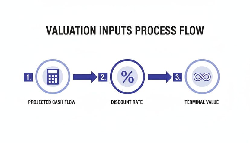
So, what are the building blocks of this financial story? A solid DCF valuation relies on a few core components that work together in your Excel model. Getting these right is the key to building a valuation you can actually trust.

This table breaks down the essential inputs and outputs of a DCF model, providing a quick reference for the key elements we will build throughout this guide.

Core Components of a DCF Model

Component	Description	Purpose in the Model
Free Cash Flow (FCF)	The cash a company generates after covering all operating expenses and capital expenditures.	This is the raw cash available to all investors (both debt and equity holders) and serves as the primary measure of a company's profitability and value.
Discount Rate (WACC)	The Weighted Average Cost of Capital, representing the blended cost of a company's debt and equity.	It's the rate we use to discount future cash flows back to the present. A higher WACC means higher risk, which lowers the present value of future cash.
Terminal Value	An estimate of the company's value beyond the explicit forecast period (usually 5-10 years).	Since a business is assumed to operate indefinitely, this captures the value of all cash flows into perpetuity, often making up a significant portion of the total valuation.

As you can see, this method forces you to think like a business owner, not just a trader. You're digging into a company's strategy, its competitive advantages, and its long-term ability to generate cash. This detailed approach is one of many powerful financial analysis techniques you can master in Excel. To dive deeper, you can explore more advanced Excel use cases for finance professionals.

A Long-Standing Analytical Tool

The DCF model isn't some new-fangled idea. Its roots go all the way back to the early 19th century. In fact, engineers in the UK coal industry were using its principles as early as 1801 to figure out if new mining projects were worth the investment.

It really gained traction after the stock market crash of 1929, as investors sought more reliable valuation methods than simplistic book value accounting. It proved to be a durable and logical way to assess a business's true worth.

A DCF analysis is useful when investing money now and expecting some rewards in the future. It finds the intrinsic value of a business, which is the present value of the free cash flow the company is expected to pay its shareholders.

By building this model yourself in Excel, you're creating a disciplined framework for making smart investment decisions. It’s all about shifting your focus from unpredictable, short-term market swings to the fundamentals of long-term value creation.

Forecasting Free Cash Flow: The Engine of Your Excel Model

Now we get to the heart of any discounted cash flow dcf model: projecting how much cash the company will actually generate. This is where your Excel skills come into play. Our goal is to forecast Unlevered Free Cash Flow (FCFF), which is the cash available to all capital providers—both stockholders and lenders—before considering financing decisions.

Typically, we’ll build this forecast out over five to ten years. This time frame is a good middle ground: it’s long enough to see the company through a full business cycle and settle into a more stable state, but not so far out that our assumptions become pure fantasy. Think of it as building a detailed, multi-year business plan right inside your spreadsheet.

Building Your Forecast From Historical Data

A credible forecast never comes out of thin air. It must be anchored in the company's historical performance. Before projecting a single number, you need to pull at least three to five years of financial statements. This data is the bedrock for every assumption you'll make in Excel.

Here are the key line items to focus on:

• Revenue: This is the starting line for everything.
• Cost of Goods Sold (COGS): The direct costs of making what you sell.
• Operating Expenses (OpEx): Think SG&A (selling, general, and administrative) costs.
• Depreciation & Amortization (D&A): Non-cash expenses that reduce your tax bill.
• Capital Expenditures (CapEx): Money spent on long-term assets like machinery or buildings.
• Changes in Net Working Capital: The annual change in current assets minus current liabilities.

Digging into this historical data helps you really understand the mechanics of the business. You’ll calculate past growth rates and operating margins, which become crucial sanity checks for your projections.

Projecting Revenue Growth and Profitability

Forecasting revenue is where art meets science. You need to build a believable story about the company's future, backed by solid, defensible assumptions. A common starting point is to calculate the historical Compound Annual Growth Rate (CAGR) and then adjust it based on industry trends, competitive landscape, and the company's own plans.

Once you have your revenue forecast, you can move on to profitability. An effective Excel technique is to assume that COGS and OpEx will remain a relatively consistent percentage of revenue, based on historical data.

For example, let's say a company has consistently hovered around a 25% operating margin. You might use that as your base assumption. In Excel, if your Year 1 projected revenue is in cell C5 and your 25% operating margin assumption is in cell B10, your formula for Earnings Before Interest and Taxes (EBIT) would be:
=C5*$B$10

Formula Explanation:

• C5 is the projected revenue for Year 1.
• $B$10 is the cell containing your operating margin assumption. The dollar signs $ make this an absolute reference, so when you drag the formula across other columns for future years, it will always refer to cell B10, keeping your assumption consistent.

Building your model with dynamic cell references like this is key. For those looking to speed up tedious tasks, many analysts find that AI can supercharge their data analysis in Excel by helping generate these kinds of complex formulas in seconds.

From EBIT to Unlevered Free Cash Flow

With your EBIT forecast in place, the next step is to make a few adjustments for non-cash items and investments to finally arrive at FCFF. This is a multi-step process where we strip out accounting conventions to get to the pure cash the business operations are producing.

The path is pretty straightforward in Excel:

1. Calculate NOPAT: Start with EBIT and subtract the projected taxes to get Net Operating Profit After Tax (NOPAT).
2. Add Back D&A: Depreciation & Amortization was an expense, but no cash actually left the business, so we add it back.
3. Subtract CapEx: Now we account for the real cash spent on long-term assets.
4. Adjust for Working Capital: Finally, we subtract any increase in Net Working Capital (or add back a decrease).

What you're left with is your Unlevered Free Cash Flow for each year in your forecast.

Key Takeaway: The whole point of forecasting FCFF is to isolate the cash generated by the core business. By ignoring the effects of debt, you get a "pure" measure of operational performance that you can value properly.

A thoughtful, well-reasoned forecast is what gives your discounted cash flow dcf model its power. It’s more than just a spreadsheet; it’s a tool that forces you to think critically about where a business is headed.

Finding Your Discount Rate and Terminal Value in Excel

Once you've forecasted the free cash flows, you have the engine of your discounted cash flow (DCF) model. But a dollar earned five years from now isn't worth a dollar today. We need a way to bring those future cash flows back to the present, and for that, we need a discount rate.

You also can't forecast forever. At some point, you must estimate the company's value for all the years beyond your forecast period. This is the Terminal Value.

Be warned: these two numbers—the discount rate and the Terminal Value—are the most powerful assumptions in your entire model. A tiny change to either one can cause your final valuation to swing wildly. Building them thoughtfully in Excel is everything.

What is the Weighted Average Cost of Capital (WACC)?

The standard discount rate for a DCF model is the Weighted Average Cost of Capital (WACC). Think of it as the average return a company needs to generate to satisfy all its investors—both the shareholders who own the equity and the lenders who hold the debt.

A high WACC indicates a riskier company. Riskier companies have their future cash flows discounted more heavily, which leads to a lower present valuation.

Here’s the classic formula we'll build in Excel:
WACC = (E / (E + D)) * Re + (D / (E + D)) * Rd * (1 – Tc)

Let’s break that down:

• E: Market Value of Equity (Market Cap)
• D: Market Value of Debt
• Re: Cost of Equity
• Rd: Cost of Debt
• Tc: The corporate tax rate

The most complex part is calculating the Cost of Equity (Re). For that, we turn to the Capital Asset Pricing Model (CAPM).

Calculating the Cost of Equity with CAPM

The CAPM formula helps us determine the return that shareholders expect for taking on the risk of investing in a particular stock compared to a "risk-free" asset.

The formula is: Re = Rf + Beta * (Rm – Rf)

To calculate this in Excel, you’ll need three inputs:

1. Risk-Free Rate (Rf): The return on a theoretically risk-free investment. Most analysts use the current yield on a long-term government bond, like the U.S. 10-Year Treasury note.
2. Beta: This measures a stock's volatility relative to the overall market. A beta of 1.0 means it moves in line with the market (e.g., the S&P 500). A beta over 1.0 means it's more volatile, while a beta under 1.0 suggests it's more stable. You can find this on financial data sites like Yahoo Finance or Bloomberg.
3. Expected Market Return (Rm): Your best estimate for the long-term annual return of the stock market. Historically, this number is often between 8% and 10%.

The (Rm - Rf) part of the formula is the Equity Market Risk Premium. It’s critical to have a good handle on the risk premium meaning, as it represents the extra compensation investors demand for taking on market risk.

Pro Tip in Excel: Create a dedicated "Assumptions" section in your spreadsheet for your WACC inputs. Give each component—Risk-Free Rate, Beta, Market Return—its own clearly labeled cell. This makes it incredibly easy to adjust these inputs later when you run a sensitivity analysis.

Capturing Value Beyond the Horizon with Terminal Value

Your detailed forecast can only go out so far—usually 5 or 10 years. The Terminal Value (TV) is your estimate of what the company will be worth at the end of that period, representing all of its cash flows from that point into perpetuity.

Don't underestimate this number. The Terminal Value often accounts for a huge portion—sometimes over 70%—of the final valuation.

There are two main ways to calculate it in Excel.

The Perpetuity Growth Model

This approach assumes the company’s cash flows will grow at a slow, steady rate forever. It works best for mature, stable businesses.

The formula is: TV = (Final Year FCFF * (1 + g)) / (WACC – g)

The key variable here is g, the perpetual growth rate. You must be conservative. A realistic rate is typically around the long-term GDP growth rate, maybe 2-3%. A higher number implies the company will eventually outgrow the entire global economy—which is impossible.

The Exit Multiple Model

This method takes a more market-based approach, assuming the company is sold at the end of your forecast for a certain multiple of a key metric, like EBITDA. This is popular for cyclical industries or when you have good data on what similar companies have recently sold for.

The formula is simple: TV = Final Year EBITDA * Exit Multiple

To choose a reasonable multiple, you would research the valuation multiples of publicly traded competitor companies or look at recent M&A deals in the same industry.

So, which one should you use? The Perpetuity Growth Model is more academic, while the Exit Multiple Model is more grounded in current market conditions. Smart analysts often calculate TV using both methods. If the two results are in the same ballpark, it gives you more confidence in your assumptions.

Assembling The Final Valuation In Excel

This is where all your hard work comes together. After forecasting cash flows, determining the discount rate, and calculating the Terminal Value, we can now assemble the final valuation summary in Excel. The goal is to arrive at a clear, defensible intrinsic value per share.

It's a journey from future cash to today's dollars, and Excel has the perfect tools to help us make that journey.

As you can see, it all boils down to three core inputs: the cash flow projections, the WACC (our discount rate), and that all-important Terminal Value.

Discounting The Cash Flows With The NPV Function

To bring all those future free cash flows into today's terms, Excel's NPV() function is your best friend. It takes your entire forecast period's cash flows and discounts each one back to the present using the WACC you calculated.

Here’s a common mistake: Excel's NPV function assumes the first cash flow you provide is one year from now. Therefore, do not include any "Year 0" cash flow inside the formula itself. It’s a subtle but critical point that can throw off your entire valuation if you get it wrong.

Let's say your WACC is in cell B2 and your projected cash flows for Years 1 through 5 are in the range C10:G10. The formula is refreshingly simple:
=NPV(B2, C10:G10)

Formula Explanation:

• B2 is the cell containing your WACC (the discount rate).
• C10:G10 is the range of cells containing your forecasted free cash flows from Year 1 to Year 5.
• This single function handles all the heavy lifting of FCF / (1+WACC)^n for each year and sums them up for you.

Getting comfortable with functions like this is a game-changer. For more tips, check out our guide on mastering Excel formulas.

Now for the Terminal Value. Since we calculated it as a single lump sum at the end of our forecast (say, Year 5), we have to discount it back to the present manually.
The formula for that is:
=TV_Cell / (1 + WACC_Cell)^Forecast_Periods

If your Terminal Value is in cell H10, WACC in B2, and you're working with a 5-year forecast, your formula would look like this: =H10 / (1 + B2)^5.

Calculating Enterprise Value

With both the present value of your forecasted cash flows and the present value of your Terminal Value ready, we can find the company's Enterprise Value (EV). Think of this as the total value of the company's core operations.

It’s just a simple sum in Excel:
Enterprise Value = PV of Forecasted FCF + PV of Terminal Value

This EV figure gives you a clean, unlevered look at the business's operational worth, independent of its debt or cash levels.

Bridging To Equity Value And Per Share Value

Enterprise Value is a crucial metric, but it’s not the price tag for the company's stock. To get to the Equity Value—the slice of the pie that actually belongs to shareholders—we need to build a "bridge" from one to the other.

This table breaks down how you get from Enterprise Value to the final Equity Value per share in your Excel model.

Enterprise Value to Equity Value Bridge
Calculation Step	Example Value	Explanation
Enterprise Value	$1,000,000	The total value of the company's operations we just calculated.
(-) Total Debt	($200,000)	Debt holders have first claim on the company's assets, so we subtract this.
(+) Cash & Equivalents	$50,000	Cash is a non-operating asset that belongs to shareholders, so it's added back.
(-) Preferred Stock	($25,000)	Preferred stock has a higher claim than common equity, so it's removed.
(-) Minority Interest	($15,000)	Value of subsidiaries not owned by the company; this portion isn't for our shareholders.
Equity Value	$810,000	This is the total value attributable to common stockholders.
(/) Diluted Shares	100,000	The total number of shares outstanding, including options and convertibles.
Value Per Share	$8.10	The final intrinsic value per share from our DCF model.

Once you have the total Equity Value, the final step is a simple division. You take that Equity Value and divide it by the company's diluted shares outstanding.

This gives you the intrinsic value per share. This is the ultimate output of your DCF analysis—a powerful number you can compare directly against the current stock price to see if the market is overvaluing or undervaluing the company.

Stress-Testing Your Excel Model With Sensitivity Analysis

A finished discounted cash flow dcf model gives you a single, precise number for what a company is worth. While that feels clean and satisfying, it's also a bit of an illusion.

That final number is incredibly sensitive to the assumptions you plugged in. A tiny tweak to your discount rate or a slight change in your growth forecast can send the valuation swinging wildly. This is why a static model is never the full picture; you must see how your result holds up when the key assumptions are pushed around.

This is exactly what sensitivity and scenario analysis are for. These techniques turn your static model into a dynamic decision-making tool in Excel. They don't just give you one answer—they show you a whole range of them, exposing the risks and opportunities hiding just beneath the surface.

Using Data Tables for Instant Sensitivity Analysis

One of the most powerful—and surprisingly underused—features in Excel for this is the Data Table. It’s a fantastic way to see how your final valuation per share reacts when you adjust two key variables at the same time. The most common inputs to test are the WACC and the terminal growth rate, because these two assumptions carry so much weight in any DCF model.

Here's how to build one in Excel:

• Set up your grid: Create a matrix on a fresh sheet. Along the top row, list a range of WACC values (e.g., 8.0%, 8.5%, 9.0%). Down the first column, do the same for your terminal growth rate (e.g., 2.0%, 2.5%, 3.0%).
• Link the output cell: In the top-left corner of this grid, create a direct link to your final "Value Per Share" calculation cell.
• Run the analysis: Highlight the entire matrix. Go to the Data tab, click What-If Analysis, and select Data Table. In the dialog box, link the "Row input cell" to the original WACC cell in your model, and link the "Column input cell" to the original terminal growth rate cell in your model.

Once you click OK, Excel instantly fills the table, calculating dozens of potential valuations. You get a visual map that immediately shows you just how fragile or robust your valuation is to changes in these crucial inputs. For those wanting to speed things up, exploring tools for AI automation in Excel can help build these kinds of complex analyses in a fraction of the time.

Why Assumptions Have a Global Impact

The weight of the discount rate isn’t just a theoretical exercise; it has huge, real-world consequences that differ from market to market. A look at historical data shows just how much risk premiums have varied across the globe.

For instance, between 1970-1990, the UK's equity premium was a hefty 6.25% (with stocks returning 14.70% vs. 8.45% for bonds). The Netherlands was lower at 4.33%, while the historically low-risk Swiss market came in at just 1.20%. These premiums feed directly into the WACC, and a higher premium means a steeper discount on future cash flows—sometimes compressing their value by 40-50% over a 10-year forecast.

This history lesson really drives home why pressure-testing your WACC is so vital. What looks like a small adjustment can reflect vastly different investor expectations and market realities.

Building Scenarios for Deeper Insight

While sensitivity tables are great for isolating one or two variables, scenario analysis lets you test a whole bundle of assumptions at once. This is perfect for modeling completely different futures for the company. The classic approach is to build out three distinct cases:

• Base Case: Your most realistic forecast, using the assumptions you believe are most likely.
• Upside Case: The optimistic view where the company exceeds all expectations.
• Downside Case: The pessimistic story where the company hits roadblocks or faces a tough economy.

Setting this up in Excel is a matter of creating a simple control panel. Use the Data Validation feature to create a dropdown menu with your three options ("Base," "Upside," "Downside"). Then, you can use a CHOOSE or nested IF function to tell your model's key drivers which assumptions to use based on the dropdown selection.

Pro Tip: If your dropdown selector is in cell A1, and cells C5, D5, and E5 hold the revenue growth rates for your Base, Upside, and Downside scenarios respectively, your formula could be: =CHOOSE(MATCH(A1,{"Base","Upside","Downside"},0),C5,D5,E5).

With this setup, you can flip between entirely different forecasts with a single click. It gives you an immediate sense of the potential range of outcomes and helps pinpoint the drivers of both risk and reward. When you combine this technique with sensitivity tables, your discounted cash flow dcf model evolves from a simple calculator into a powerful framework for making smart decisions.

Speed Up Your DCF Workflow with AI in Excel

Building a discounted cash flow dcf model from scratch is a grind. It's filled with repetitive tasks, complex formulas, and tiny details where one slip-up can invalidate the entire valuation. But what if you could automate the grunt work and focus on strategic thinking? That’s exactly what integrating AI directly into Excel enables.

You can offload the mechanical bits and spend your time on what actually matters—the assumptions that drive your final valuation.

Forget wrestling with nested formulas or spending an hour cleaning historical data. With an AI assistant integrated into Excel, you can use simple, plain-English commands to get things done. Think of it as telling your spreadsheet what to do, like asking it to instantly organize messy financial statements, write the correct WACC formula for you, or build a sensitivity analysis chart on the fly.

Let AI Handle the Heavy Lifting

This isn't about making your financial expertise obsolete; it’s about supercharging it. The AI becomes your co-pilot, handling the tedious steps so you can put your brainpower toward actual analysis.

Here are a few practical examples in Excel:

• Data Cleaning: Instead of manual cleanup, just tell the AI, "Remove duplicates, standardize all date formats, and fill any blank cells with the column average." Your raw data is ready in seconds.
• Formula Generation: Can't remember the exact syntax for a complex function? No problem. Just ask, "Generate the Excel formula to calculate the present value of the terminal value in cell G20, using the WACC in B5 and a 5-year forecast period." The correct formula appears instantly.
• Visualization: Creating charts is just as easy. A simple request like, "Build a waterfall chart showing the bridge from Enterprise Value to Equity Value using the data in range A15:B20," gives you a professional-looking visual instantly.

This fundamentally changes how you work. When you automate the mechanics, you free up time to think critically about growth assumptions, the competitive landscape, and risk factors—the elements that truly create an insightful valuation.

The speed you gain is a massive advantage. If you're curious about how this works, you can learn more about bringing the power of AI into your Excel workflows with tools built for this purpose.

For a broader look at how advanced tech is changing the investment world, check out this guide on Mastering AI in Venture Capital. Adopting these tools isn't just about efficiency; it's about making your analysis sharper and more reliable.

Got Questions About DCF Models? We've Got Answers.

As you get your hands dirty building DCF models in Excel, a few questions always seem to pop up. Let's tackle some of the most common ones to clear up any confusion and sharpen your understanding.

What's the Achilles' Heel of a DCF Model?

The biggest weakness of a DCF model is its extreme sensitivity to its own assumptions. It's a classic "garbage in, garbage out" situation.

A tiny tweak to the discount rate or the terminal growth rate can cause the final valuation to swing wildly. This makes the entire model heavily dependent on the analyst's judgment and the quality of their inputs.

This is exactly why you can't just build one model and call it a day. Stress-testing with sensitivity and scenario analysis in Excel isn't just a nice-to-have; it's a must-do. It shows you how fragile your valuation is and which assumptions are driving the most risk.

How Far Out Should I Forecast?

A five-year forecast period is the industry standard, and for many stable companies, it works just fine.

However, if you're analyzing a high-growth startup or a business in a highly cyclical industry, pushing the forecast out to 7-10 years is often a smarter move. You need to give the company enough time on paper to mature and settle into a more predictable, stable growth pattern before you apply a terminal value calculation.

Can a DCF Actually Give Me a Negative Value?

Absolutely. It might seem strange, but a negative valuation is a real and often telling result.

If your projections show a company consistently burning through cash with negative free cash flows, the math will reflect that reality. The present value of all those future cash outflows can easily result in a negative Enterprise Value. This is usually a massive red flag, signaling serious issues with the company's financial health or its entire business model.

---

Building a robust discounted cash flow dcf model doesn't have to be a grind. With Elyx.AI, you can stop wrestling with messy data and complex formulas. Let our autonomous AI agent take over the heavy lifting—from data prep to final charts—so you can focus on what really matters: the strategic insights.

Ready to see it in action? Start your free trial at Elyx.AI and build your next DCF model in a fraction of the time.