Mastering the DCF Model in Excel: A Practical Guide

If you're serious about valuation, the Discounted Cash Flow (DCF) model is your bread and butter. It's the standard for figuring out what a company is truly worth by looking at the cash it’s expected to generate in the future. In essence, a DCF model in Excel helps you turn a company's story into a number, giving you a solid, data-backed foundation for any investment decision. This guide provides a practical, step-by-step approach to building a robust DCF from scratch using Excel.

Why Mastering the DCF Model in Excel Is a Core Skill

Building a DCF isn't just a classroom drill; it's how professionals in the real world decide what a company is worth. For anyone working in or aspiring to a career in finance, mastering the DCF in Excel is non-negotiable. It's a fundamental technique used everywhere—from equity research and M&A to internal corporate strategy.

The whole point of a DCF analysis is to project a company’s future cash flows and then pull those future values back to today's dollars. It’s built on a simple, powerful idea: a dollar today is worth more than a dollar tomorrow.

The Power of Excel for Financial Modeling

Despite all the fancy software out there, Excel is still king for financial modeling. Why? Its flexibility and ubiquity are unmatched. Excel's grid is perfectly designed for laying out financial statements, assumptions, and calculations in a way that's easy to follow, audit, and adjust.

A well-built DCF model in Excel accomplishes a few critical things:

• Clarity and Transparency: It forces you to lay out every single assumption, showing exactly how each one impacts the final valuation.
• Dynamic Analysis: You can easily build in sensitivity tables and different scenarios. What happens to the valuation if the growth rate drops by 1%? Or if interest rates rise? A good model tells you instantly.
• Decision Support: Ultimately, the model gives you a quantitative basis for making big calls. Is this stock a buy? Does this acquisition make sense? The model helps you answer that.

A well-informed valuation enables managers to make wiser decisions regarding capital budgeting and strategic planning. Outside the company, investors need to measure value to assess the risks and returns of their investments with greater confidence.

Moving Beyond Theory to Practical Application

Enough with the theory. This guide will walk you through the practical, hands-on steps of building a real DCF. We'll cover how to structure your workbook, forecast cash flows, nail down the right discount rate, and calculate terminal value.

I'll also show you how modern AI assistants can handle the grunt work, freeing you up to focus on the high-level insights that actually matter. There are plenty of other powerful Excel use cases that can make your entire workflow more efficient.

Laying the Groundwork for a Bulletproof Excel Model

A great valuation doesn't start with complex formulas. It starts with a clean, organized, and error-resistant spreadsheet. Before you even think about forecasting cash flows, the most important thing you can do is build a solid foundation. This structure not only makes your DCF model easier to build, but it also makes it transparent and easy for others to follow your work.

Think of your Excel file like the blueprint for a house. A sloppy layout leads to confusion, errors, and a model no one can trust. But a well-structured one? It’s intuitive, scalable, and professional.

Structuring Your DCF Workbook

I can't stress this enough: separate your model into dedicated worksheets. Each tab should have a single, clear purpose. This modular approach is the best way to prevent your model from becoming a tangled, single-sheet nightmare of formulas and inputs. It also makes debugging and future updates a breeze.

Let's walk through the essential worksheet layout that I've seen used in professional settings, from investment banking to corporate finance.

---

Essential Worksheet Layout for a DCF Model

Here’s a summary of the recommended tabs and their specific purpose in a professional DCF model. Sticking to this structure will make your life much easier.

Worksheet Tab Name	Purpose and Key Content	Best Practice Tip
Assumptions	This is the control panel for your entire model. It houses all key drivers like revenue growth, margins, tax rates, and the WACC.	Never hard-code an assumption directly into a formula. Always link back to this single, centralized tab.
Historical Financials	Input at least three to five years of the company's past financial data, typically pulled from 10-K and 10-Q reports.	Keep the formatting identical to the source reports. This makes it simple to check your work and trace numbers back to their origin.
Forecast	This is where you project the three financial statements (Income Statement, Balance Sheet, Cash Flow) based on your drivers.	Build your forecast logic so that it directly pulls from the Assumptions tab. This way, you can change a driver once and see it ripple through the model.
DCF Valuation	Here's where the magic happens. You'll calculate Unlevered Free Cash Flow (UFCF), Terminal Value, and discount everything to find Enterprise Value.	Clearly lay out each step of the calculation, from EBIT to NOPAT to UFCF. Don't try to cram it all into one massive formula.
Sensitivity Analysis	This tab tests how your valuation changes when key assumptions (like WACC or growth rates) are flexed up and down.	Use Excel's Data Table feature to automate this. It's a game-changer for understanding which assumptions truly drive the valuation.

---

This organized, multi-tab approach is the industry standard for a reason—it works. It keeps things clean and auditable.

Formatting for Clarity and Auditability

One of the most common sources of error in any financial model is mixing up inputs and calculations. A simple color-coding system is a small detail that signals a high level of professionalism and care, making your model instantly understandable.

A well-formatted model tells a clear story. By color-coding cells, you create a visual language that separates hard-coded inputs from dynamic formula outputs, drastically reducing the risk of manual error and making the model's logic transparent.

Here's the standard convention nearly every analyst uses:

• Blue Text: For all hard-coded inputs and assumptions. If you type a number directly into a cell, make it blue.
• Black Text: For all formulas and calculations that reference cells within the same worksheet.
• Green Text: For formulas that link to other worksheets in the same workbook. This makes it incredibly easy to trace dependencies across your model.

This discipline is critical. Proficiency in DCF modeling is a top skill, cited by 85% of investment bankers. Best practices like clear labeling have been shown to boost model accuracy by as much as 40%—a huge deal when you consider that an estimated 30% of models contain formula bugs.

With a clean structure, clear formatting, and solid historicals in place, you are now ready to start building the core calculations. Mastering this setup will also help you apply the same logic to other tasks, like those we cover in our guide to creating powerful Excel formulas.

Forecasting Unlevered Free Cash Flow with Confidence

With a clean Excel workbook ready to go, it's time to dive into the core of the valuation: forecasting the Unlevered Free Cash Flow (UFCF). This is where you transform the company's story—its strategy, market position, and growth plans—into cold, hard numbers. The most credible forecasts are always built on a solid foundation of logical, defensible assumptions, which we call forecast drivers.

Everything starts with revenue. Don't just pull a growth number out of thin air. Your revenue assumptions need to be grounded in reality, reflecting the company’s own history and the broader trends of its industry. I always start by analyzing historical growth rates, but then I'll layer in an understanding of the total market size and the competitive landscape.

This diagram lays out the essential groundwork for getting your model set up correctly—organizing your data, formatting the sheets for clarity, and pulling the right inputs from financial filings.

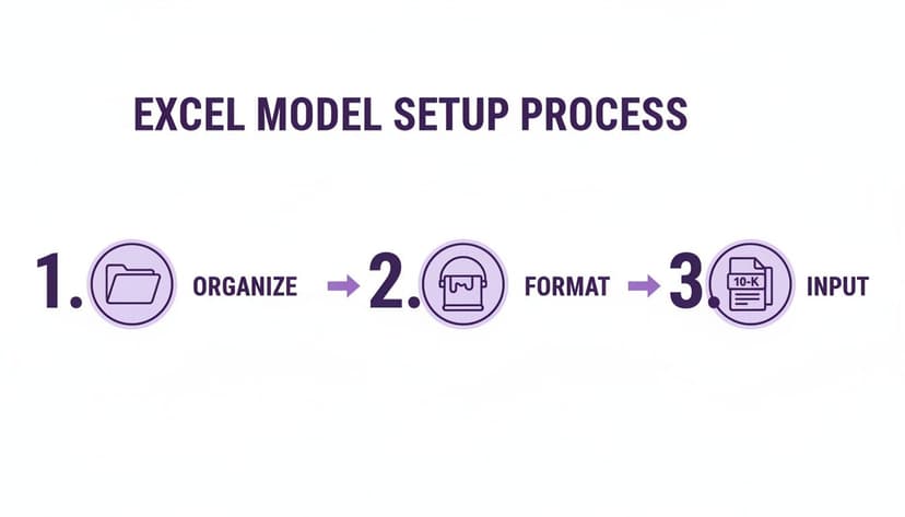
Getting this initial setup right is crucial. A well-organized model with clearly labeled tabs and clean formatting makes the entire process smoother and ensures your work is easy to follow and audit later.

Projecting Down the Income Statement

Once your top-line revenue forecast is in place, the next step is to work your way down the income statement. This means projecting the major expense lines to ultimately arrive at operating profit. A very common and practical approach is to forecast these expenses as a percentage of revenue, using historical averages or management guidance as your guide.

For instance, if a company's Cost of Goods Sold (COGS) has consistently hovered around 60% of its revenue for the last five years, it's a safe bet to keep it there in your forecast. Of course, if management announced a major supply chain overhaul, you'd want to adjust that assumption. The same logic holds true for Selling, General & Administrative (SG&A) expenses.

Calculating Net Operating Profit After Tax (NOPAT)

The first major calculation on our journey to UFCF is Net Operating Profit After Tax (NOPAT). Think of NOPAT as the company's potential cash earnings if it were completely debt-free. It gives you a pure, unobstructed view of the business's core operational efficiency, free from the noise of its financing decisions.

The formula itself is pretty simple:

NOPAT = EBIT × (1 – Tax Rate)

In an Excel formula, if your Earnings Before Interest and Taxes (EBIT) for the first forecast year is in cell C10 and your tax rate assumption (let's say 21%) is on a separate 'Assumptions' tab in cell B5, you would write:

=C10 * (1 - Assumptions!$B$5)

Let's break down this formula:

• C10 refers to the cell containing your EBIT for the given period.
• Assumptions!$B$5 refers to the cell on your "Assumptions" worksheet that holds the tax rate.
• The $ signs create an absolute reference. This is a small but critical detail that locks the tax rate cell, so when you drag your formula across the forecast period, it continues to reference the correct tax rate.

From NOPAT to Unlevered Free Cash Flow

NOPAT is a great measure of profitability, but it isn't cash in the bank. To get to the actual Unlevered Free Cash Flow, we need to make a few key adjustments for non-cash expenses and the investments the company makes to keep the lights on and grow.

Here's the standard path to calculate UFCF:

1. Start with NOPAT: This is your after-tax operating profit.
2. Add back Depreciation & Amortization (D&A): D&A is a non-cash expense that lowered your EBIT, so you have to add it back to get closer to a cash figure.
3. Subtract Capital Expenditures (CapEx): This accounts for the real cash the company spends on long-term assets like factories, equipment, or technology.
4. Subtract the Change in Net Working Capital (NWC): This adjustment reflects the cash tied up in day-to-day operations, like inventory and accounts receivable.

In practice, analysts almost always forecast these explicit free cash flows for a 5-10 year period. After that, we calculate a terminal value because we assume the business will operate indefinitely. This two-stage approach has become the gold standard, with the DCF model in Excel powering well over 90% of valuations in investment banking.

The Real-World Impact of Small Assumption Changes

Never underestimate how much your drivers impact the final valuation. Let’s imagine you're building a DCF model in Excel for a retail company. A seemingly small tweak, like bumping up the projected gross margin by just 1% because you believe they’re getting better at managing their supply chain, can create a massive ripple effect.

That single percentage point flows straight down to EBIT, which then increases NOPAT and boosts every single UFCF figure in your forecast. When you discount all that extra cash back to today, that tiny change could easily increase the company's valuation by 5-10% or even more. It's a stark reminder of how sensitive these models are.

This sensitivity is exactly why building a robust model with clear, traceable assumptions is non-negotiable. Manually digging through historical data to find these trends can be a grind, but specialized tools for AI data analysis in Excel can help you quickly identify key historical patterns to build a more informed set of forecast drivers.

Nailing Your WACC and Terminal Value

Once you’ve projected a company’s future cash flows, the next crucial job is figuring out what those future dollars are actually worth today. This is where we get into two of the most critical—and honestly, most debated—parts of any DCF model: the discount rate and the terminal value. Getting these right is what separates a good valuation from a flimsy one.

The discount rate we'll use is the Weighted Average Cost of Capital (WACC). Think of it as the company's blended cost for all the money it uses to run its business, from both debt and equity, weighted accordingly. Simply put, WACC is the minimum return a company has to earn just to keep its investors and lenders happy. It’s the hurdle that every dollar of future cash flow has to clear.

Breaking Down the WACC Calculation

To get to our WACC, we need to figure out the cost of each type of capital and then weight them based on how much of each the company uses.

The textbook formula looks like this:

WACC = (E/V × Re) + [(D/V × Rd) × (1 – Tc)]

Let's quickly translate what each of those pieces means for your Excel sheet:

• (E/V): This is just the proportion of equity in the company's capital structure. You calculate it as the Market Value of Equity divided by the Total Market Value of Equity and Debt.
• Re: This is the Cost of Equity—the return shareholders demand. Most of the time, we calculate this using the Capital Asset Pricing Model (CAPM).
• (D/V): The flip side of the coin, this is the proportion of debt in the capital structure.
• Rd: This is the Cost of Debt, or the effective interest rate the company is paying.
• Tc: The corporate tax rate. We multiply the cost of debt by (1 – Tc) because interest payments are tax-deductible. This "tax shield" effectively lowers the true cost of borrowing.

Building this out in your model means you'll need to source the risk-free rate (a 10-year government bond yield is a good proxy), the market risk premium, and the company's beta for the CAPM piece. My advice? Lay each of these components out in its own cell on your 'Assumptions' tab. It keeps things clean and easy to audit later.

Why Terminal Value Is So Important

Next, we have to deal with a simple business reality: most companies are expected to keep running long after our 5 or 10-year forecast ends. The Terminal Value (TV) is our attempt to capture the value of the company for all those years beyond our explicit projection, rolled into a single number.

Here’s a fact that surprises a lot of newcomers to DCF modeling: the terminal value often accounts for 60-80% of a company's total enterprise value. This really drives home how sensitive your final valuation is to the long-term assumptions you make. If you get this part wrong, your entire valuation could be off by 20-30% or even more. If you want to dig deeper into this, you can review some expert DCF model breakdowns to see just how much this number moves the needle.

There are two main ways analysts tackle this crucial calculation.

Method 1: The Perpetuity Growth Model

This is the classic academic approach. It assumes the company’s free cash flows will grow at a steady, constant rate into perpetuity. The whole game here is picking a realistic and conservative long-term growth rate (g).

A defensible perpetual growth rate should never be higher than the long-term growth rate of the overall economy (think GDP). I typically use something between 2.0% and 3.0%. Anything higher suggests the company will one day be bigger than the entire economy—a clear impossibility.

The Excel formula for this is pretty straightforward:

= (Final Year UFCF * (1 + g)) / (WACC - g)

In this formula:

• Final Year UFCF is the Unlevered Free Cash Flow from your last forecast year.
• g is your chosen perpetual growth rate.
• WACC is your discount rate.

The formula takes the final year's cash flow, grows it by one period at the long-term rate g, and then divides that by the difference between your WACC and g to find its present value.

Method 2: The Exit Multiple Method

This method is much more common in the world of investment banking and private equity because it mirrors how a business might actually be sold. You just assume the company is sold at the end of your forecast period for a multiple of a key financial metric, usually EBITDA.

To do this, you need to research what similar companies are trading for in the public markets or what they've recently been acquired for. For example, if comparable businesses are trading at an average of 8.0x EV/EBITDA, you’d apply that multiple to your company's projected EBITDA in its final forecast year.

In Excel, it looks like this:

= Final Year Projected EBITDA * Selected Exit Multiple

So, which one should you use? It really depends on the company and the industry. For a stable, mature business, the perpetuity growth model often feels right. For a high-growth company or one in a cyclical industry, an exit multiple can provide a more realistic, market-based anchor for its value. In practice, many of the best analysts calculate the terminal value using both methods as a way to sanity-check their assumptions and create a valuation range.

Deriving Valuation and Running a Sensitivity Analysis

Alright, you've done the heavy lifting. The cash flows are projected, the terminal value is calculated, and now it's time for the payoff. This is where we pull everything together to find the company's intrinsic value.

All that detailed forecasting and assumption-setting was for this moment: combining the explicit forecast period with the terminal value and discounting it all back to today’s dollars. This process turns abstract forecasts into a tangible, present-day valuation, which is the entire point of building a DCF model in Excel.

Calculating Enterprise Value with Excel's NPV Function

The first thing we need to do is find the present value of all those future cash flows. That includes the cash flow for each year of your explicit forecast (say, years 1-10) and the terminal value, which bundles up all cash flows from year 11 into infinity.

Excel’s NPV function is perfect for this, but be careful—its name is a bit misleading. It doesn’t actually calculate the Net Present Value; it calculates the present value of a series of future cash flows.

The syntax is simple: NPV(rate, value1, [value2], ...)

Let’s imagine your WACC is in cell C5, your projected Unlevered Free Cash Flows for years 1 through 10 are in the range D15:M15, and your terminal value is sitting in cell M16.

Here’s how you’d structure the formula:

=NPV(C5, D15:M15) + M16 / (1 + C5)^10

Let's break that down quickly:

• NPV(C5, D15:M15) takes all the cash flows from your main forecast period (years 1-10) and discounts them back to today's value (year 0).
• M16 / (1 + C5)^10 handles the terminal value separately. Since the terminal value is calculated as of the end of the forecast period (year 10), we have to discount it back manually for 10 years to find its present value.

Add those two parts together, and you get the company’s Enterprise Value (EV).

Bridging to Equity Value and Implied Share Price

So, what is Enterprise Value? It’s the total value of a company's core business operations available to all its investors, both debt and equity holders. But we usually want to know what the company is worth to just the shareholders. To get there, we need to build a "bridge" from EV to Equity Value.

The calculation is pretty standard:

1. Start with Enterprise Value: This is the total value we just calculated.
2. Add Cash and Cash Equivalents: Cash is a non-operating asset, so we add it back.
3. Subtract Total Debt: This includes both short-term and long-term borrowings.
4. Subtract Minority Interest: If the company owns subsidiaries but doesn't own 100% of them, we subtract the value of the portion it doesn't own.

The final number is the Equity Value. To get to the bottom line—the implied price per share—you just divide that Equity Value by the company’s fully diluted shares outstanding. This gives you a concrete price you can compare to what the stock is trading at in the market. If your implied price is much higher, your model is telling you the stock might be undervalued. At its core, a DCF helps you figure out how to value your business from the ground up.

The Power of Sensitivity Analysis

Here's a crucial reality check: a DCF model produces a single number, but that number is built on a stack of assumptions. What if your WACC is off by 0.5%? What if that long-term growth rate is a little too optimistic?

A single-point valuation is fragile. A valuation range, on the other hand, is robust. This is where sensitivity analysis becomes the most important tool in your DCF model in Excel.

A valuation is not a number; it's a narrative backed by numbers. Sensitivity analysis lets you test that narrative under different conditions, revealing which assumptions have the most impact and transforming your static model into a dynamic decision-making tool.

Excel has a fantastic feature called a Data Table that’s built for exactly this. It lets you create a two-variable grid showing how your implied share price (the output) changes when two of your key drivers (the inputs)—like WACC and the perpetuity growth rate—move around.

You set it up with a range of WACC values down one axis and a range of growth rates across the other. Link the table to your implied share price cell, and Excel instantly populates the grid, showing you dozens of potential outcomes at a glance. It's a powerful way to visualize your valuation's pressure points.

If you get stuck on the formulas for setting this up, a tool like Elyx AI can be a real time-saver. You can see how its AI formula generator can help speed up complex tasks like these.

How AI Can Accelerate Your DCF Modeling

Once you've gotten your hands dirty and built a DCF model in Excel from the ground up, the next step is to find ways to work smarter. The core principles of valuation don't change, but the tools we use are getting much, much better. AI assistants built right into Excel can literally save you hours of tedious, manual work.

Think about it. Instead of digging through help forums to remember the right formula syntax or meticulously building charts piece by piece, you can just use simple, plain-English commands. This lets you stop wrestling with the mechanics of Excel and start focusing on the strategic assumptions that actually drive a meaningful valuation.

From Manual Formulas to Natural Language Prompts

Let's take a common task: projecting revenue. The old way involves finding your historical data, using a specific formula to calculate the compound annual growth rate (CAGR), and then carefully applying that rate across your forecast period. It's not hard, but it's fiddly.

With an AI assistant like Elyx, you can just type what you want directly into your spreadsheet:

"Calculate the 5-year revenue CAGR from the 'Historical Financials' tab and use it to project revenue for the next 5 years in the 'Forecast' tab."

The AI instantly generates and applies the correct formula. This frees you up to do the real work: thinking critically about the output. Is that historical growth rate really the best assumption going forward? Should it be tweaked based on new market trends? That's where an analyst adds real value.

Automating Complex Analyses

The power of AI goes well beyond just creating formulas. Remember the sensitivity analysis we walked through? Building a two-variable data table is a classic Excel power-move, but it’s also notoriously tricky. One wrong cell reference and the whole thing breaks.

Now, you can hand that entire task off with a clear instruction. For instance, you could tell the AI:

"Create a sensitivity table showing how the implied equity value per share changes. Use WACC ranging from 7% to 11% (in 0.5% steps) and a perpetuity growth rate between 2.0% and 4.0% (in 0.25% steps)."

The AI agent builds the table, links it to the right model outputs, and formats it for you. This doesn’t just save a ton of time; it also cuts out the risk of human error on a complex setup.

By automating the repetitive parts of financial modeling, you get to spend more of your brainpower on what really matters: figuring out the story the numbers are telling. You can learn more about the capabilities of a dedicated AI assistant for Excel and see how it could fit into your workflow.

Common Questions About Building DCF Models

Even with a great template in hand, you're bound to run into a few tricky questions when building a DCF model. Let's tackle some of the most common hurdles I've seen trip up analysts, which will help you sidestep these frequent mistakes.

How Do I Choose the Right Forecast Period?

This is a classic judgment call. How far out is too far? The industry standard for most valuations is a 5-10 year forecast period. That's usually long enough to see a company through a full business cycle but short enough that your assumptions don't veer into pure guesswork.

Think about the company's lifecycle. For a stable, mature business with predictable growth, a five-year forecast might be all you need. But if you're looking at a high-growth tech startup or a company in a highly cyclical industry, you'll likely need a 10-year view to capture its full potential before it settles into a more predictable, stable growth phase.

What Are the Biggest Mistakes to Avoid?

Honestly, the most damaging errors I see in DCF models rarely come from a busted formula. They almost always stem from flawed assumptions.

Here are the top culprits to watch out for:

• Overly Optimistic Growth: This is the big one. Plugging in a terminal growth rate that's way too high is probably the most common mistake out there. Remember, this rate should not exceed the long-term growth rate of the overall economy.
• Mismatched Discount Rate: It's critical to match your cash flow to your discount rate. For instance, using the cost of equity to discount unlevered free cash flows will throw your entire valuation off.
• Logical Inconsistencies: Your assumptions need to tell a coherent story. If your model shows a sudden, massive jump in profit margins without any real-world justification, that should be a major red flag.

The real strength of a DCF model isn't its complexity; it's the defensibility of its assumptions. A tiny error in a key driver like WACC or the terminal growth rate can have a huge ripple effect on the final valuation. Always double-check your inputs.

Can I Build a DCF Without a Full 3-Statement Model?

Yes, you absolutely can. It's possible to create a simplified or "standalone" DCF by making direct assumptions for the key inputs needed to calculate Unlevered Free Cash Flow, such as capital expenditures and changes in Net Working Capital.

While a fully integrated 3-statement model is the gold standard because of its internal consistency, a standalone DCF is fantastic for a quick ‘back-of-the-envelope’ valuation when you're short on time.

---

Ready to stop wrestling with formulas and start focusing on strategy? With Elyx AI, you can automate everything from data cleaning to chart creation with simple, natural language commands. Try our AI-powered Excel add-in and see how much time you can save. Get started with your free trial at https://getelyxai.com.